弘前データ1:法定検診との関係
ここではまずデータの視覚化を行い,概要をつかむ. 次節から階層モデリングを目指す.
4/27/2025
まずは簡単な回帰を実行
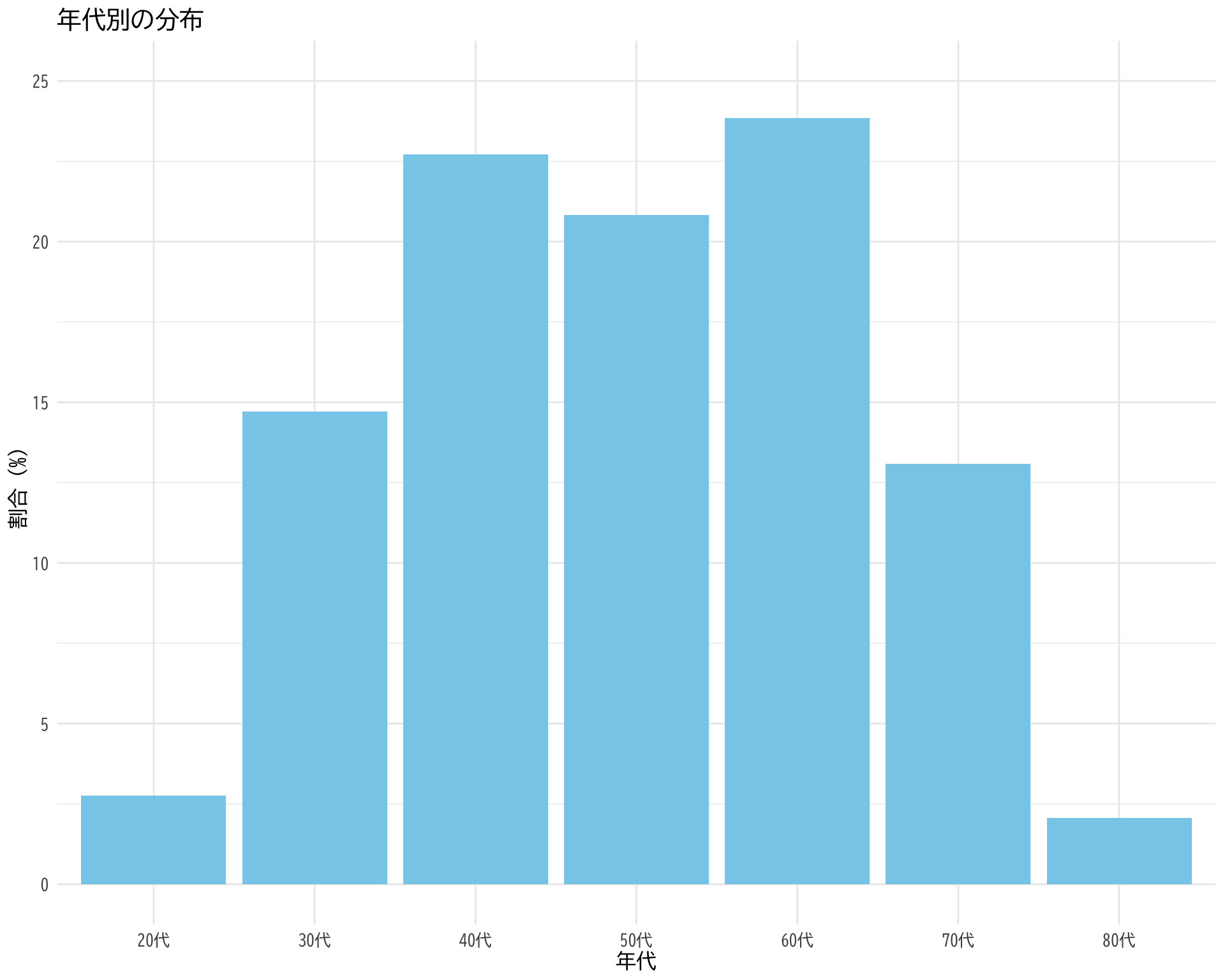
ここでは BP と LAB の関係のモデリングを行う. hirosaki3.qmd では \(\Sigma\)-FLC と LOX-1 の関係をモデリングする. ここでは簡単な回帰を実行した. 年代により逆転する変動係数が推定された.
kable(head(df))| 受診日年齢 | 性別 | Weight | BP | BP備考 | 判別式 | LOX-1_H | LAB_H | LOX-index_H | タイプ | 多様性 | item1 | item2 | item3 | item4 | item5 | item6 | item7 | item8 | item9 | item10 | item11 | item12 | item13 | item14 | item15 | item16 | item17 | item18 | BP_A_flag | 年代 | 活気 | イライラ感 | 疲労感 | 不安感 | 抑うつ感 |
|---|---|---|---|---|---|---|---|---|---|---|---|---|---|---|---|---|---|---|---|---|---|---|---|---|---|---|---|---|---|---|---|---|---|---|---|
| 64 | 2 | 54.2 | 1.08 | ABDG | -2.880 | 86 | 2.6 | 224 | B | 2 | 2 | 2 | 2 | 1 | 1 | 1 | 1 | 1 | 1 | 1 | 1 | 1 | 1 | 1 | 1 | 1 | 1 | 1 | 1 | 60代 | 3 | 1 | 1 | 1 | 1 |
| 48 | 2 | 52.7 | 0.47 | B | -3.343 | 75 | 2.2 | 165 | B | 2 | 2 | 2 | 2 | 2 | 2 | 2 | 4 | 3 | 2 | 3 | 2 | 2 | 2 | 2 | 1 | 2 | 3 | 2 | 0 | 40代 | 3 | 3 | 4 | 3 | 3 |
| 53 | 2 | 64.8 | 0.67 | BDG | -2.727 | 55 | 2.8 | 154 | A | 1 | 3 | 1 | 1 | 1 | 1 | 2 | 3 | 3 | 3 | 2 | 2 | 2 | 2 | 2 | 1 | 1 | 1 | 1 | 0 | 50代 | 4 | 2 | 4 | 3 | 2 |
| 46 | 1 | 76.3 | 1.10 | NA | -2.974 | 136 | 3.8 | 517 | B | 2 | 2 | 3 | 3 | 2 | 2 | 2 | 1 | 1 | 2 | 2 | 2 | 1 | 2 | 2 | 1 | 1 | 1 | 1 | 0 | 40代 | 2 | 3 | 2 | 3 | 2 |
| 65 | 1 | 72.4 | 0.88 | D | -7.338 | 58 | 2.3 | 133 | C | 2 | 3 | 3 | 3 | 2 | 2 | 2 | 1 | 1 | 1 | 2 | 1 | 1 | 1 | 1 | 1 | 1 | 1 | 1 | 0 | 60代 | 2 | 3 | 1 | 2 | 1 |
| 30 | 1 | 59.5 | 0.76 | NA | -2.776 | 46 | 2.2 | 101 | B | 2 | 2 | 2 | 2 | 3 | 4 | 3 | 3 | 3 | 3 | 4 | 4 | 3 | 3 | 3 | 3 | 3 | 1 | 1 | 0 | 30代 | 3 | 5 | 4 | 5 | 4 |
mdf <- df[, c(1:11, 30:36)]
colnames(mdf) <- gsub("_H$", "", colnames(mdf))
colnames(mdf) <- gsub("LOX-1", "LOX", colnames(mdf))  # LOX-1をLOXに
colnames(mdf) <- gsub("LOX-index", "LI", colnames(mdf))  # LOX-indexをLIに
kable(head(mdf))| 受診日年齢 | 性別 | Weight | BP | BP備考 | 判別式 | LOX | LAB | LI | タイプ | 多様性 | BP_A_flag | 年代 | 活気 | イライラ感 | 疲労感 | 不安感 | 抑うつ感 |
|---|---|---|---|---|---|---|---|---|---|---|---|---|---|---|---|---|---|
| 64 | 2 | 54.2 | 1.08 | ABDG | -2.880 | 86 | 2.6 | 224 | B | 2 | 1 | 60代 | 3 | 1 | 1 | 1 | 1 |
| 48 | 2 | 52.7 | 0.47 | B | -3.343 | 75 | 2.2 | 165 | B | 2 | 0 | 40代 | 3 | 3 | 4 | 3 | 3 |
| 53 | 2 | 64.8 | 0.67 | BDG | -2.727 | 55 | 2.8 | 154 | A | 1 | 0 | 50代 | 4 | 2 | 4 | 3 | 2 |
| 46 | 1 | 76.3 | 1.10 | NA | -2.974 | 136 | 3.8 | 517 | B | 2 | 0 | 40代 | 2 | 3 | 2 | 3 | 2 |
| 65 | 1 | 72.4 | 0.88 | D | -7.338 | 58 | 2.3 | 133 | C | 2 | 0 | 60代 | 2 | 3 | 1 | 2 | 1 |
| 30 | 1 | 59.5 | 0.76 | NA | -2.776 | 46 | 2.2 | 101 | B | 2 | 0 | 30代 | 3 | 5 | 4 | 5 | 4 |
library(ggplot2)
mini_df <- df[df$BP_A_flag == 0, c("BP", "LAB_H")]
colnames(mini_df) <- c("BP", "LAB")

ggplot(mini_df, aes(x = LAB, y = BP)) +
  geom_point(alpha = 0.5, color = "skyblue") +
  geom_smooth(method = "lm", color = "red", se = TRUE) +
  theme_minimal() +
  labs(title = "LAB と BP の相関",
       x = "LAB",
       y = "BP") +
  theme(
    text = element_text(family = "BIZUDGothic-Regular", size = 12),
    axis.text = element_text(size = 34),
    axis.title = element_text(size = 45),
    plot.title = element_text(size = 45)
  ) +
  # 両軸のスケールを同じに
  coord_fixed(ratio = 1) +
  # 軸の範囲を-3から3に設定(標準偏差の±3倍程度)
  scale_x_continuous(limits = c(0, 5)) +
  scale_y_continuous(limits = c(0, 2.5))
`geom_smooth()` using formula = 'y ~ x'Warning: Removed 55 rows containing non-finite values (`stat_smooth()`).Warning: Removed 55 rows containing missing values (`geom_point()`).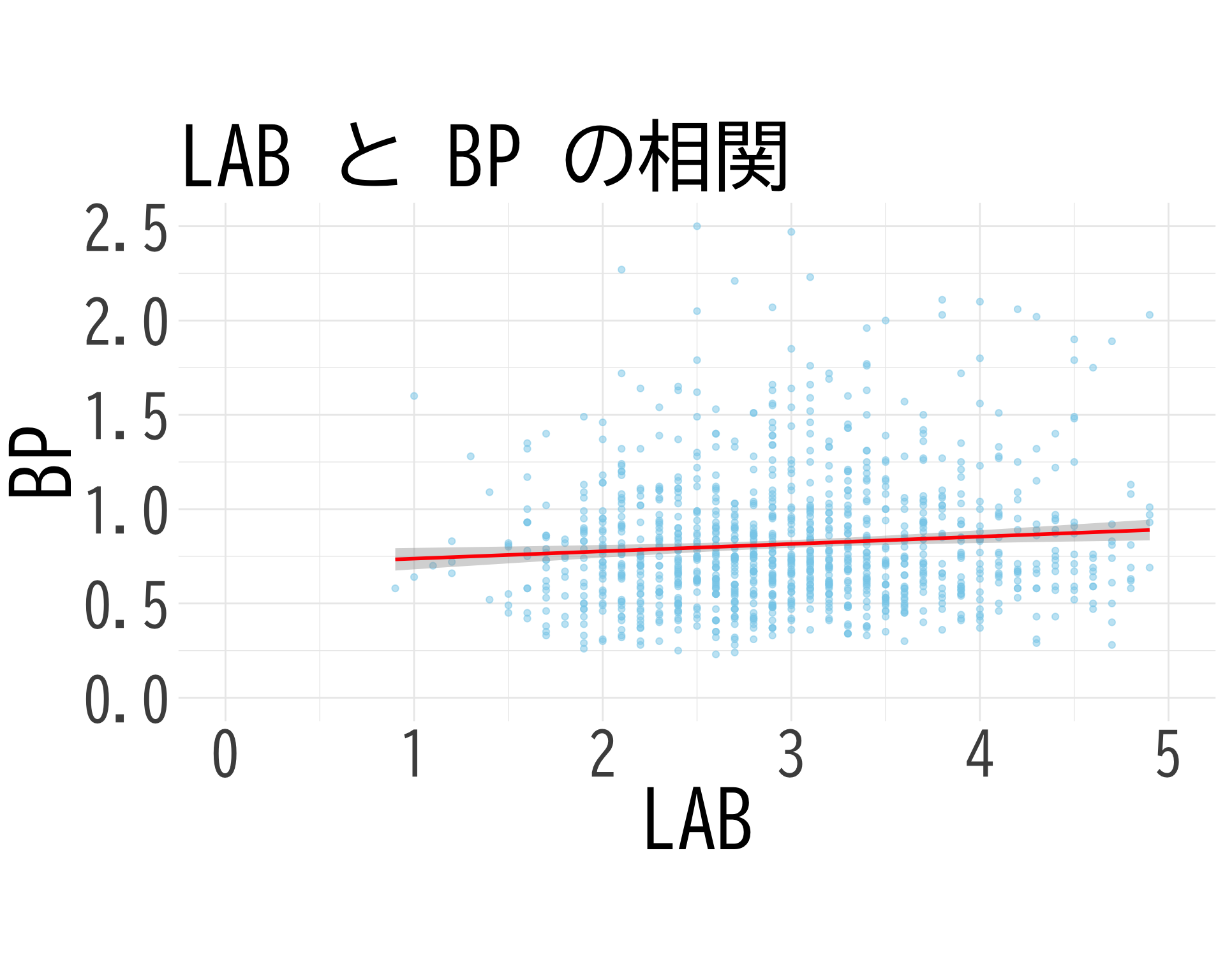
# 30代のデータのみを抽出
mini_df_30s <- df[df$BP_A_flag == 0 & df$年代 == "30代", c("BP", "LAB_H")]
colnames(mini_df_30s) <- c("BP", "LAB")

# プロット
ggplot(mini_df_30s, aes(x = LAB, y = BP)) +
  geom_point(alpha = 0.5, color = "skyblue") +
  geom_smooth(method = "lm", color = "red", se = TRUE) +
  theme_minimal() +
  labs(title = "30 代での相関",
       x = "LAB",
       y = "BP") +
  theme(
    text = element_text(family = "BIZUDGothic-Regular", size = 12),
    axis.text = element_text(size = 34),
    axis.title = element_text(size = 45),
    plot.title = element_text(size = 45)
  ) +
  coord_fixed(ratio = 1) +
  scale_x_continuous(limits = c(1, 4.5)) +
  scale_y_continuous(limits = c(0, 2.0))
`geom_smooth()` using formula = 'y ~ x'Warning: Removed 6 rows containing non-finite values (`stat_smooth()`).Warning: Removed 6 rows containing missing values (`geom_point()`).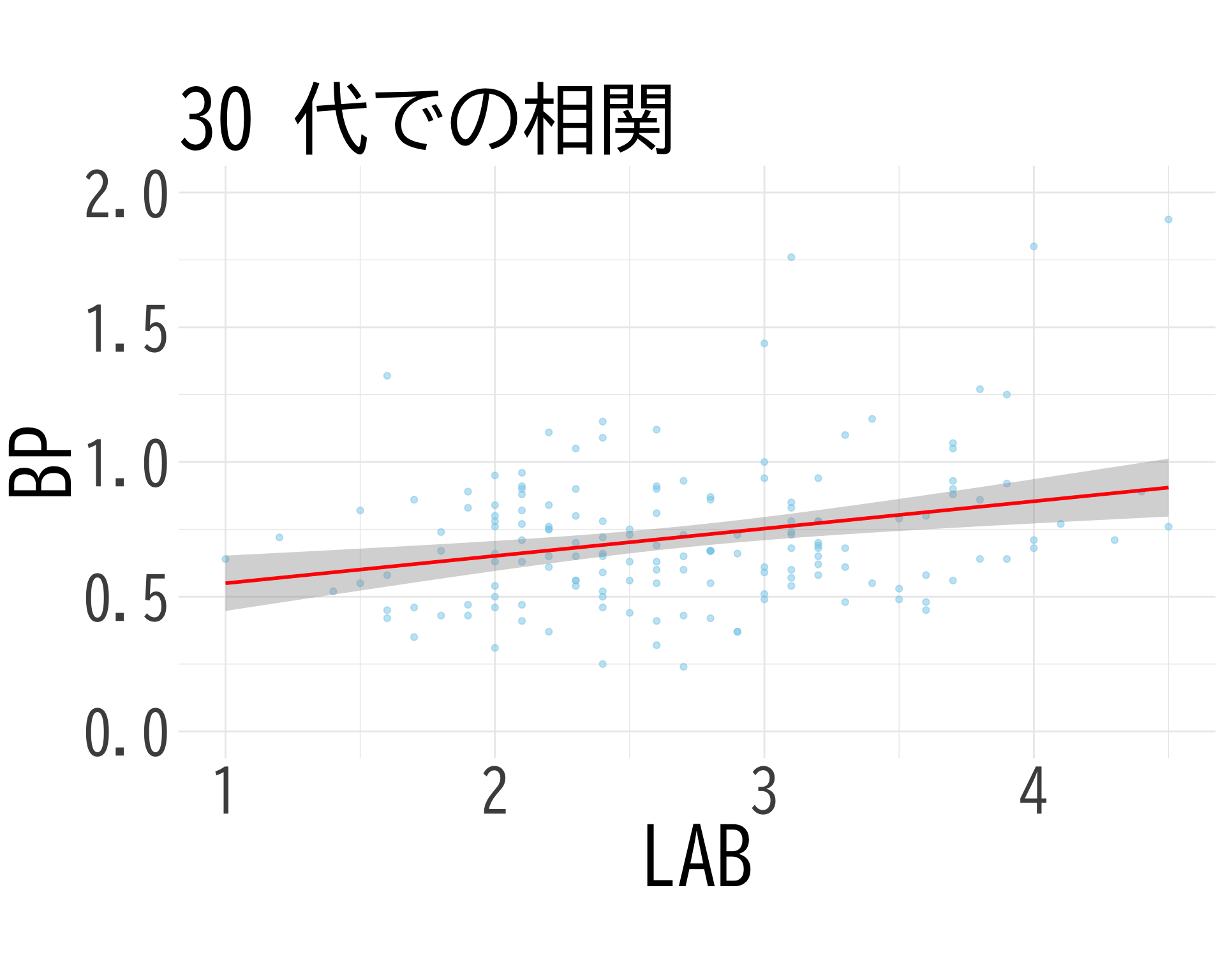
ggsave("LAB_BP_30.png", bg="white")Saving 10 x 8 in image
`geom_smooth()` using formula = 'y ~ x'Warning: Removed 6 rows containing non-finite values (`stat_smooth()`).
Removed 6 rows containing missing values (`geom_point()`).# 70代のデータのみを抽出
mini_df_70s <- df[df$BP_A_flag == 0 & df$年代 == "70代", c("BP", "LAB_H")]
colnames(mini_df_70s) <- c("BP", "LAB")
# プロット
ggplot(mini_df_70s, aes(x = LAB, y = BP)) +
geom_point(alpha = 0.5, color = "skyblue") +
geom_smooth(method = "lm", color = "red", se = TRUE) +
theme_minimal() +
labs(title = "70 代での相関",
x = "LAB",
y = "BP") +
theme(
text = element_text(family = "BIZUDGothic-Regular", size = 12),
axis.text = element_text(size = 34),
axis.title = element_text(size = 45),
plot.title = element_text(size = 45)
) +
coord_fixed(ratio = 1) +
scale_x_continuous(limits = c(2, 5.5)) +
scale_y_continuous(limits = c(0, 2.0))`geom_smooth()` using formula = 'y ~ x'Warning: Removed 10 rows containing non-finite values (`stat_smooth()`).Warning: Removed 10 rows containing missing values (`geom_point()`).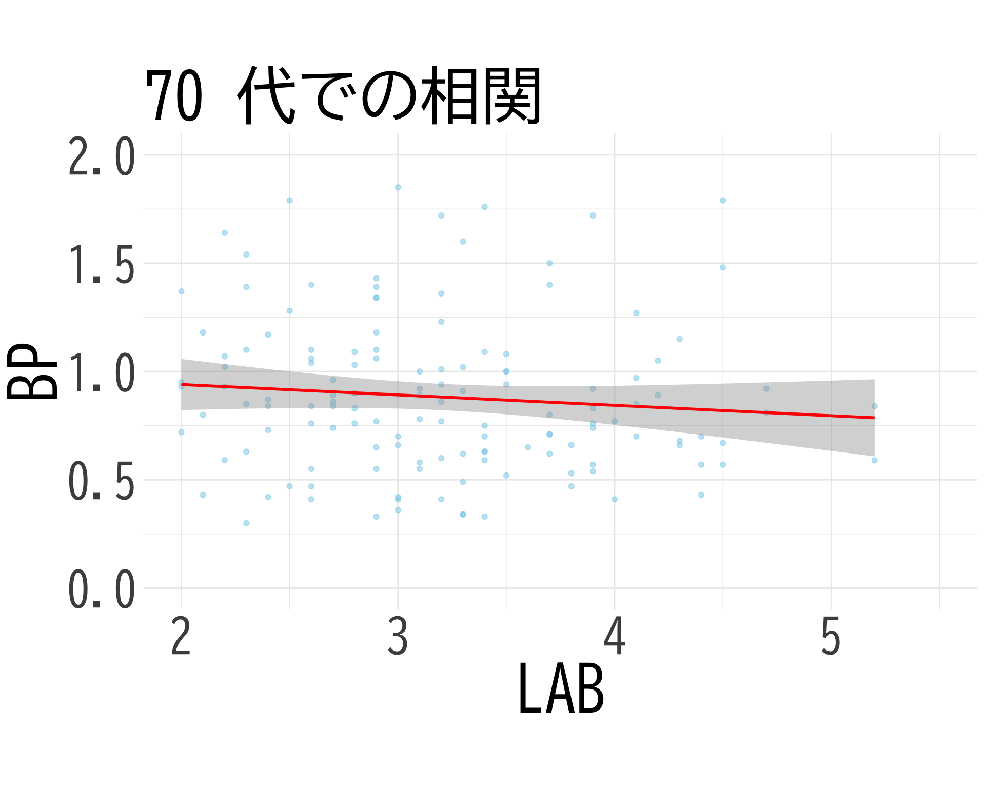
ggsave("LAB_BP_70.png", bg="white")Saving 10 x 8 in image
`geom_smooth()` using formula = 'y ~ x'Warning: Removed 10 rows containing non-finite values (`stat_smooth()`).
Removed 10 rows containing missing values (`geom_point()`).normalize <- function(x) {
(x - mean(x, na.rm = TRUE)) / sd(x, na.rm = TRUE)
}
# 新しいデータフレームを作成し、必要な列を標準化
df_norm <- data.frame(
BP = normalize(mdf$BP),
LAB = normalize(mdf$LAB),
LOX = normalize(mdf$LOX),
LI = normalize(mdf$LI)
)library(brms)Warning: パッケージ 'brms' はバージョン 4.3.1 の R の下で造られました 要求されたパッケージ Rcpp をロード中です Loading 'brms' package (version 2.21.0). Useful instructions
can be found by typing help('brms'). A more detailed introduction
to the package is available through vignette('brms_overview').
次のパッケージを付け加えます: 'brms' 以下のオブジェクトは 'package:stats' からマスクされています:
arformula <- bf(
BP ~ 1 + LAB + LOX + LI
)
fit <- brm(
formula,
data = df_norm,
family = gaussian(),
chains = 4,
iter = 4000,
cores = 4
)Warning: Rows containing NAs were excluded from the model.Compiling Stan program...Start samplingplot(fit)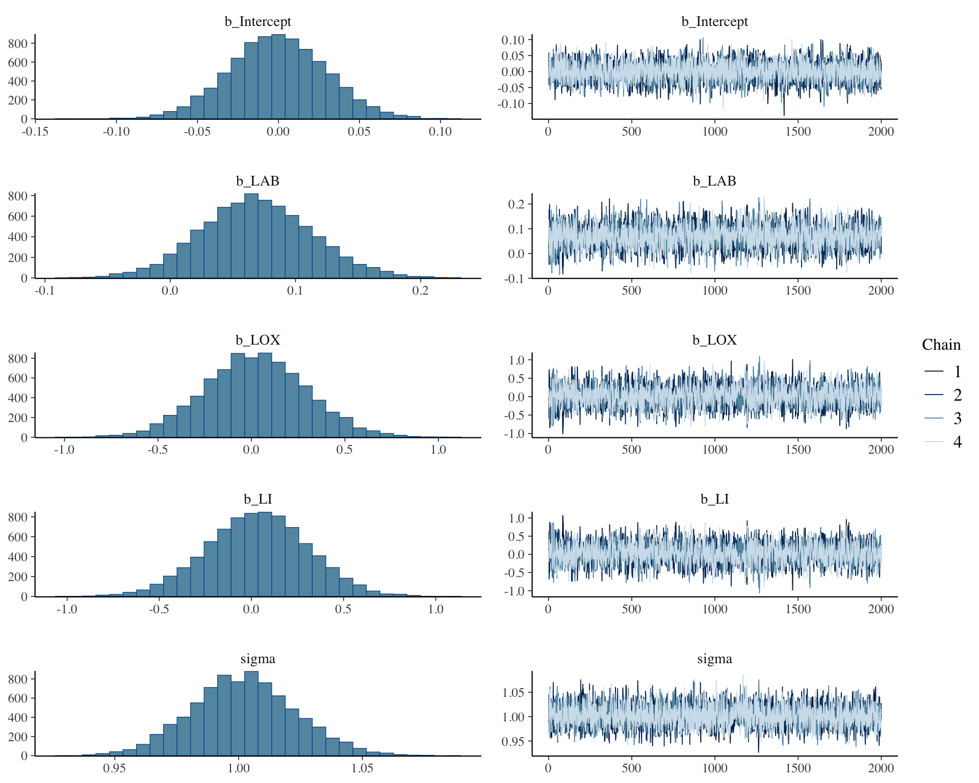
summary(fit) Family: gaussian
Links: mu = identity; sigma = identity
Formula: BP ~ 1 + LAB + LOX + LI
Data: df_norm (Number of observations: 1124)
Draws: 4 chains, each with iter = 4000; warmup = 2000; thin = 1;
total post-warmup draws = 8000
Regression Coefficients:
Estimate Est.Error l-95% CI u-95% CI Rhat Bulk_ESS Tail_ESS
Intercept -0.00 0.03 -0.06 0.06 1.00 4640 3828
LAB 0.07 0.04 -0.02 0.16 1.00 3408 3991
LOX 0.02 0.27 -0.51 0.56 1.00 3020 3463
LI 0.03 0.28 -0.51 0.57 1.00 3007 3645
Further Distributional Parameters:
Estimate Est.Error l-95% CI u-95% CI Rhat Bulk_ESS Tail_ESS
sigma 1.00 0.02 0.96 1.04 1.00 4564 4601
Draws were sampled using sampling(NUTS). For each parameter, Bulk_ESS
and Tail_ESS are effective sample size measures, and Rhat is the potential
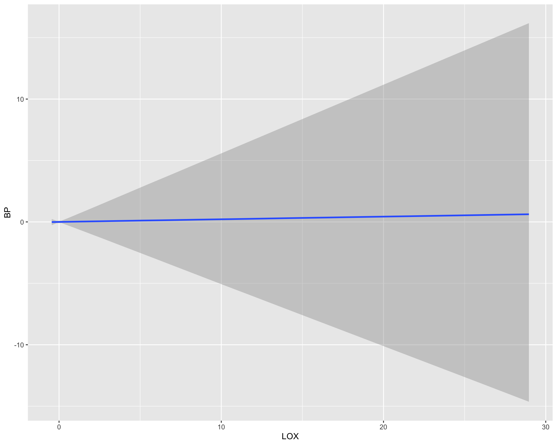
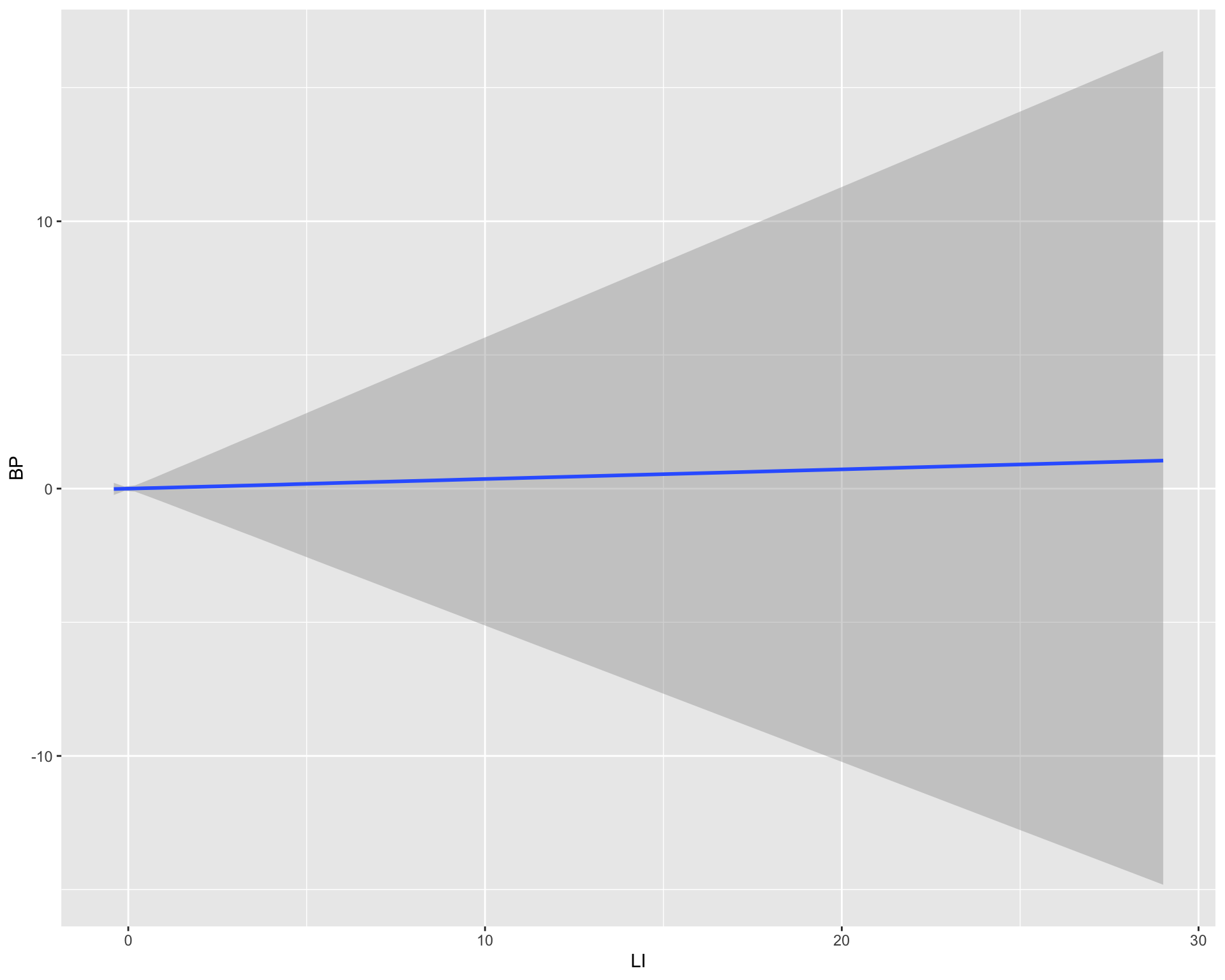
scale reduction factor on split chains (at convergence, Rhat = 1).conditional_effects(fit)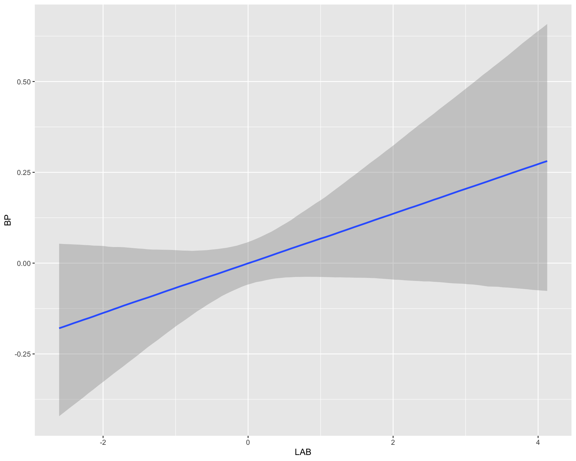
そもそも BP の背景濃度が年代別に違うならば,切片項も年代ごとに変動させる必要があるか?
library(brms)

formula <- bf(
  BP ~ 1 + (1 + LAB | 年代)
)
fit <- brm(
  formula,
  data = mdf,
  family = gaussian(),
  chains = 4,
  iter = 8000,
  cores = 4
)
Warning: Rows containing NAs were excluded from the model.Compiling Stan program...Start samplingWarning: There were 353 divergent transitions after warmup. See
https://mc-stan.org/misc/warnings.html#divergent-transitions-after-warmup
to find out why this is a problem and how to eliminate them.Warning: Examine the pairs() plot to diagnose sampling problems# データフレームの作成
plot_data <- data.frame(
年代 = 1:7, # 数値として扱う(20代=1, 30代=2, ...)
効果 = ranef(fit)$年代[,1,"LAB"]
)
# プロット
ggplot(plot_data, aes(x = 年代, y = 効果)) +
# 回帰直線
geom_smooth(method = "lm", color = "black", se = TRUE) +
# 大きな赤い点
geom_point(color = "#E15759", size = 4) +
theme_minimal() +
labs(title = "年代別のランダム効果(LAB)",
x = "年代",
y = "LAB のランダム係数") +
theme(
text = element_text(family = "BIZUDGothic-Regular", size = 16),
axis.text = element_text(size = 34),
axis.title = element_text(size = 45),
plot.title = element_text(size = 45)
) +
geom_hline(yintercept = 0, linetype = "dashed", color = "black") +
scale_x_continuous(
breaks = 1:7,
labels = c("20代", "30代", "40代", "50代", "60代", "70代", "80代")
) +
coord_fixed(ratio = 70)`geom_smooth()` using formula = 'y ~ x'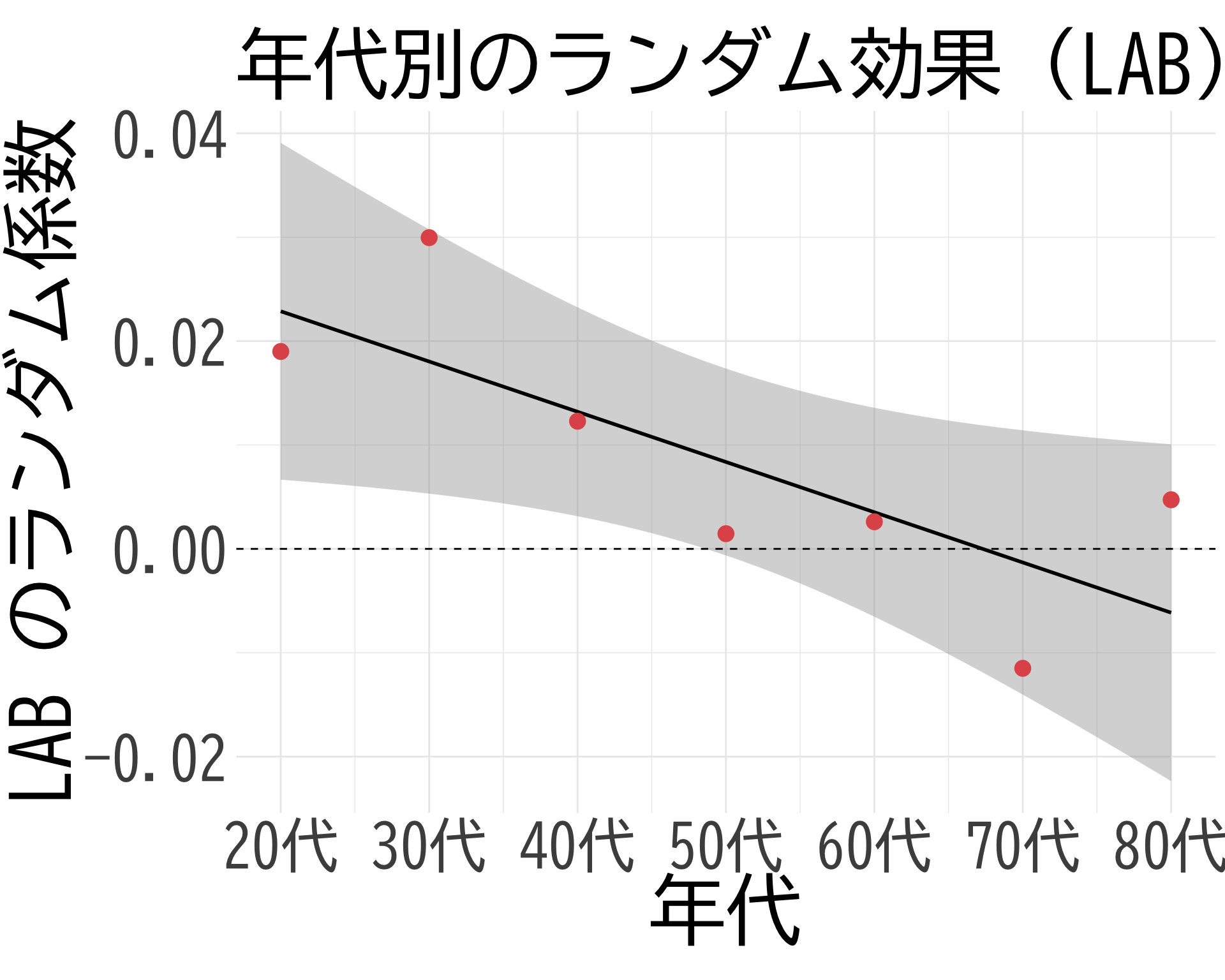
# ggsave("LABの年代効果.png", bg="white")library(brms)
formula <- bf(
BP ~ 1 + (LOX | 年代)
)
fit <- brm(
formula,
data = mdf,
family = gaussian(),
chains = 4,
iter = 8000,
cores = 4
)Warning: Rows containing NAs were excluded from the model.Compiling Stan program...Start samplingWarning: There were 207 divergent transitions after warmup. See
https://mc-stan.org/misc/warnings.html#divergent-transitions-after-warmup
to find out why this is a problem and how to eliminate them.Warning: Examine the pairs() plot to diagnose sampling problems