library(readxl)
library(knitr)
df <- readRDS("df.rds")
df <- df[is.na(df$`BP備考`), ]
kable(head(df))
| 3 |
4 |
46 |
1 |
76.3 |
1.10 |
1.95 |
NA |
-2.974 |
136 |
3.8 |
517 |
B |
2 |
26.0 |
2 |
NA |
40代 |
2 |
3 |
2 |
3 |
2 |
| 5 |
6 |
30 |
1 |
59.5 |
0.76 |
0.64 |
NA |
-2.776 |
46 |
2.2 |
101 |
B |
2 |
19.5 |
2 |
NA |
30代 |
3 |
5 |
4 |
5 |
4 |
| 6 |
7 |
51 |
1 |
76.6 |
1.69 |
2.58 |
NA |
-2.377 |
78 |
3.2 |
250 |
B |
2 |
25.5 |
2 |
NA |
50代 |
3 |
3 |
3 |
3 |
2 |
| 7 |
8 |
47 |
2 |
43.2 |
0.56 |
0.55 |
NA |
-3.048 |
40 |
2.7 |
108 |
B |
2 |
16.7 |
2 |
NA |
40代 |
2 |
1 |
2 |
2 |
1 |
| 9 |
10 |
39 |
1 |
61.9 |
0.52 |
0.64 |
NA |
-3.165 |
54 |
2.4 |
130 |
B |
2 |
21.3 |
2 |
NA |
30代 |
3 |
3 |
3 |
3 |
3 |
| 10 |
11 |
55 |
1 |
61.0 |
0.89 |
2.64 |
NA |
-3.708 |
60 |
3.1 |
186 |
E |
1 |
22.9 |
1 |
NA |
50代 |
3 |
2 |
2 |
1 |
1 |
df_IRT_long <- readRDS("df_IRT_long.rds")
df_IRT_long <- df_IRT_long[df_IRT_long$FLCΣ > 0, ]
kable(head(df_IRT_long))
| 1 |
2 |
0.47 |
0.81 |
B |
2 |
活気 |
3 |
0 |
| 2 |
2 |
0.47 |
0.81 |
B |
2 |
イライラ感 |
3 |
0 |
| 3 |
2 |
0.47 |
0.81 |
B |
2 |
疲労感 |
4 |
1 |
| 4 |
2 |
0.47 |
0.81 |
B |
2 |
不安感 |
3 |
0 |
| 5 |
2 |
0.47 |
0.81 |
B |
2 |
抑うつ感 |
3 |
0 |
| 11 |
4 |
1.10 |
1.95 |
B |
2 |
活気 |
2 |
0 |
library(ggplot2)
library(dplyr)
 以下のオブジェクトは 'package:stats' からマスクされています:

    filter, lag
 以下のオブジェクトは 'package:base' からマスクされています:

    intersect, setdiff, setequal, union
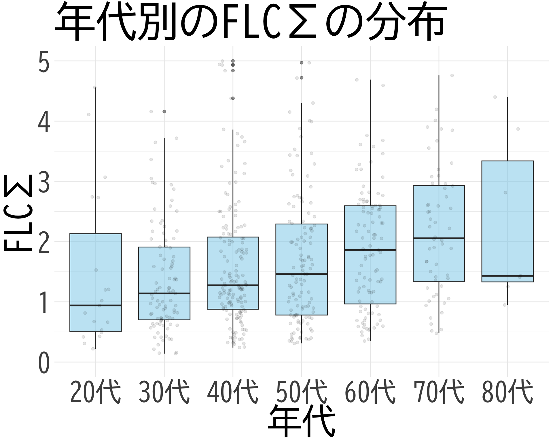
# 男性のデータ
df_plot <- df %>%
  filter(!is.na(FLCΣ), !is.na(年代))

# 2つのプロットを横に並べる
ggplot(df_plot, aes(x = 年代, y = FLCΣ)) +
  geom_boxplot(fill = "skyblue", alpha = 0.5) +
  geom_jitter(width = 0.2, alpha = 0.1) +
  theme_minimal() +
  labs(title = "年代別のFLCΣの分布",
       x = "年代",
       y = "FLCΣ") +
  theme(
    text = element_text(family = "BIZUDGothic-Regular", size = 12),
    axis.text = element_text(size = 34),
    axis.title = element_text(size = 45),
    title = element_text(size = 45)
  ) +
  scale_y_continuous(limits = c(0,5))
Warning: Removed 28 rows containing non-finite values (`stat_boxplot()`).
Warning: Removed 28 rows containing missing values (`geom_point()`).
library(ggplot2)
library(dplyr)
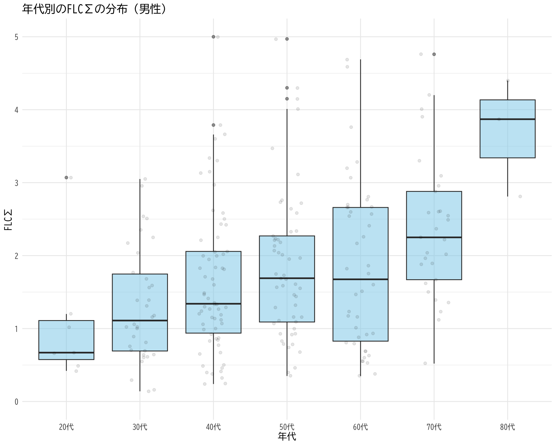
# 男性のデータ
df_male <- df %>%
filter(!is.na(FLCΣ), !is.na(年代), sex == 1)
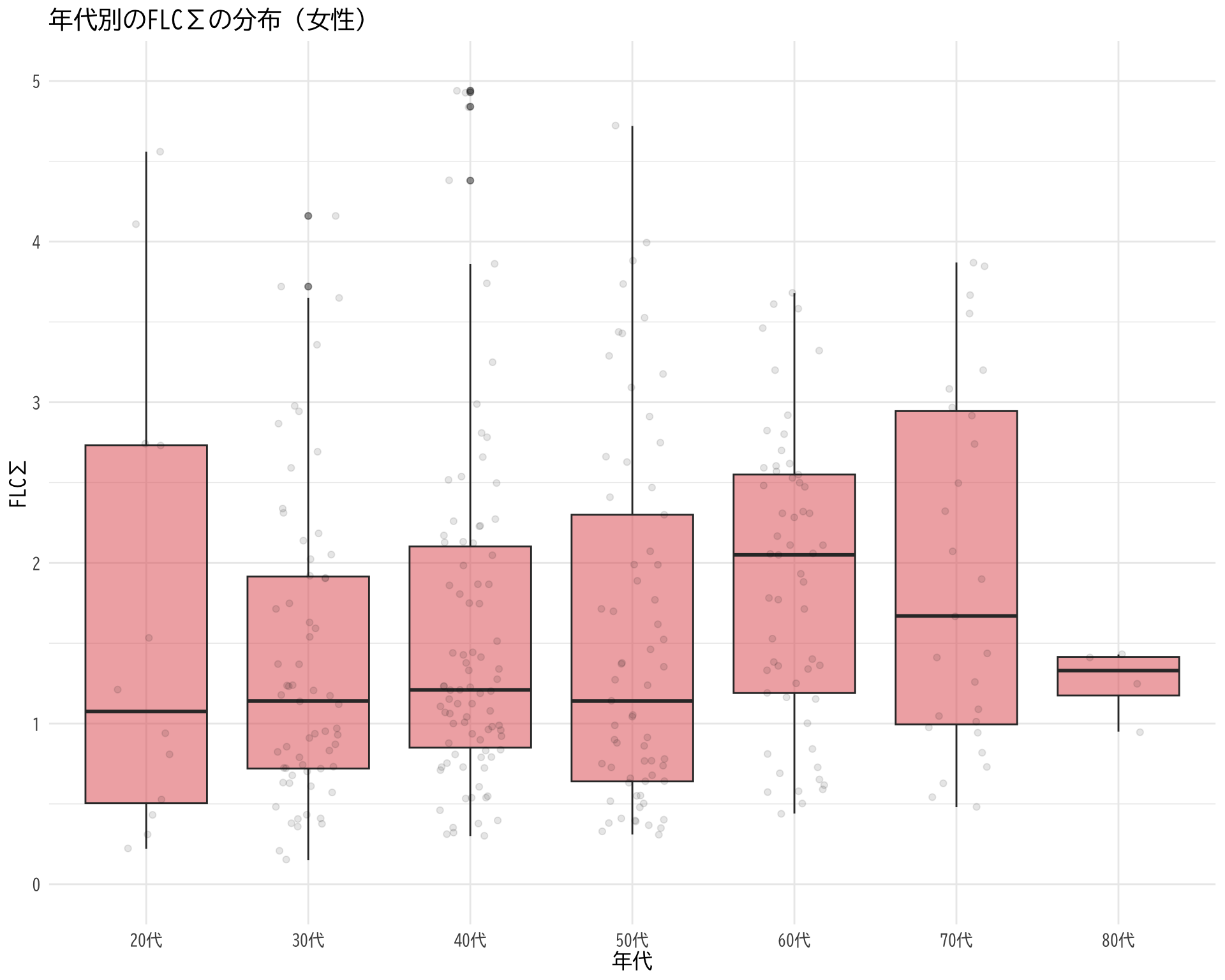
# 女性のデータ
df_female <- df %>%
filter(!is.na(FLCΣ), !is.na(年代), sex == 2)
# 2つのプロットを横に並べる
plot1 <- ggplot(df_male, aes(x = 年代, y = FLCΣ)) +
geom_boxplot(fill = "skyblue", alpha = 0.5) +
geom_jitter(width = 0.2, alpha = 0.1) +
theme_minimal() +
labs(title = "年代別のFLCΣの分布(男性)",
x = "年代",
y = "FLCΣ") +
theme(
text = element_text(family = "BIZUDGothic-Regular", size = 12)
) +
scale_y_continuous(limits = c(0,5))
plot2 <- ggplot(df_female, aes(x = 年代, y = FLCΣ)) +
geom_boxplot(fill = "#E15759", alpha = 0.5) +
geom_jitter(width = 0.2, alpha = 0.1) +
theme_minimal() +
labs(title = "年代別のFLCΣの分布(女性)",
x = "年代",
y = "FLCΣ") +
theme(
text = element_text(family = "BIZUDGothic-Regular", size = 12)
) +
scale_y_continuous(limits = c(0,5))
plot1
Warning: Removed 11 rows containing non-finite values (`stat_boxplot()`).
Warning: Removed 11 rows containing missing values (`geom_point()`).
Warning: Removed 17 rows containing non-finite values (`stat_boxplot()`).
Warning: Removed 17 rows containing missing values (`geom_point()`).