64
2
54.2
1.08
ABDG
-2.880
86
2.6
224
B
2
2
2
2
1
1
1
1
1
1
1
1
1
1
1
1
1
1
1
1
60代
3
1
1
1
1
48
2
52.7
0.47
B
-3.343
75
2.2
165
B
2
2
2
2
2
2
2
4
3
2
3
2
2
2
2
1
2
3
2
0
40代
3
3
4
3
3
53
2
64.8
0.67
BDG
-2.727
55
2.8
154
A
1
3
1
1
1
1
2
3
3
3
2
2
2
2
2
1
1
1
1
0
50代
4
2
4
3
2
46
1
76.3
1.10
NA
-2.974
136
3.8
517
B
2
2
3
3
2
2
2
1
1
2
2
2
1
2
2
1
1
1
1
0
40代
2
3
2
3
2
65
1
72.4
0.88
D
-7.338
58
2.3
133
C
2
3
3
3
2
2
2
1
1
1
2
1
1
1
1
1
1
1
1
0
60代
2
3
1
2
1
30
1
59.5
0.76
NA
-2.776
46
2.2
101
B
2
2
2
2
3
4
3
3
3
3
4
4
3
3
3
3
3
1
1
0
30代
3
5
4
5
4
とりあえず記述
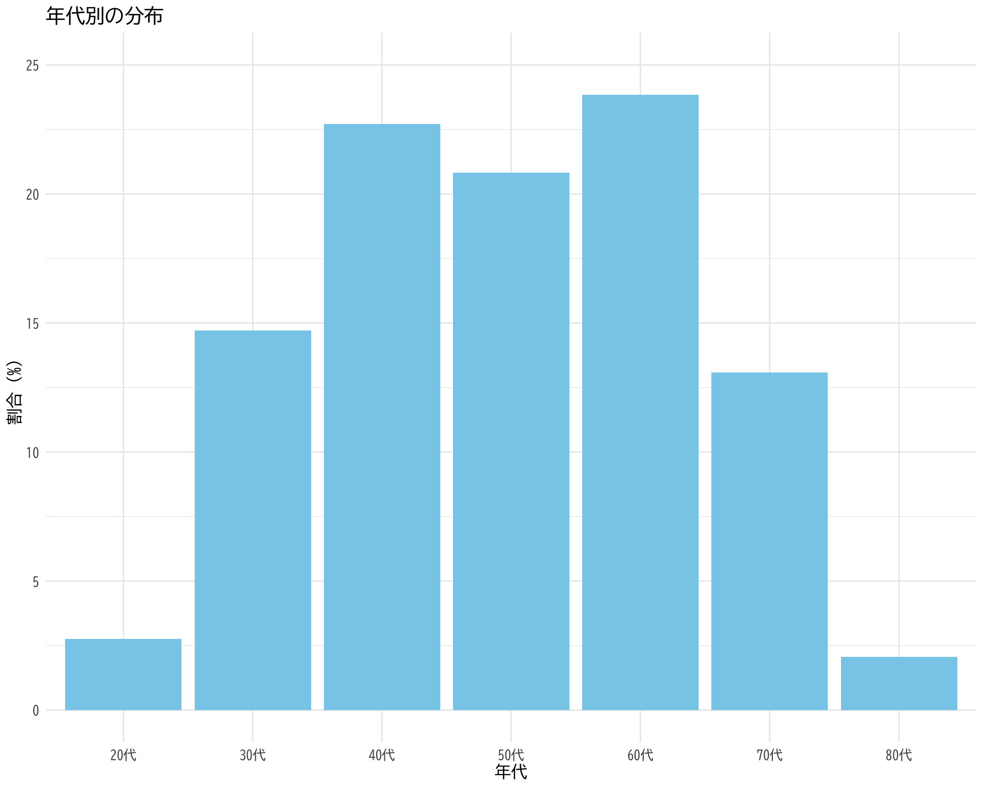
年代ごとの人数分布
prop.table (table (df$ 年代)) * 100
     20代      30代      40代      50代      60代      70代      80代
 2.753873 14.716007 22.719449 20.826162 23.838210 13.080895  2.065404
library (ggplot2)<- as.data.frame (prop.table (table (df$ 年代)) * 100 )colnames (age_dist) <- c ("年代" , "割合" )# ggplotでプロット ggplot (age_dist, aes (x = 年代, y = 割合)) + geom_bar (stat = "identity" , fill = "skyblue" ) + theme_minimal () + labs (title = "年代別の分布" ,x = "年代" ,y = "割合(%)" ) + theme (text = element_text (family = "BIZUDGothic-Regular" , size = 12 ),# axis.text = element_text(size = 34), # axis.title = element_text(size = 45), # title = element_text(size = 45) + scale_y_continuous (limits = c (0 , 25 ))# ggsave("age_dist.png", bg="white")
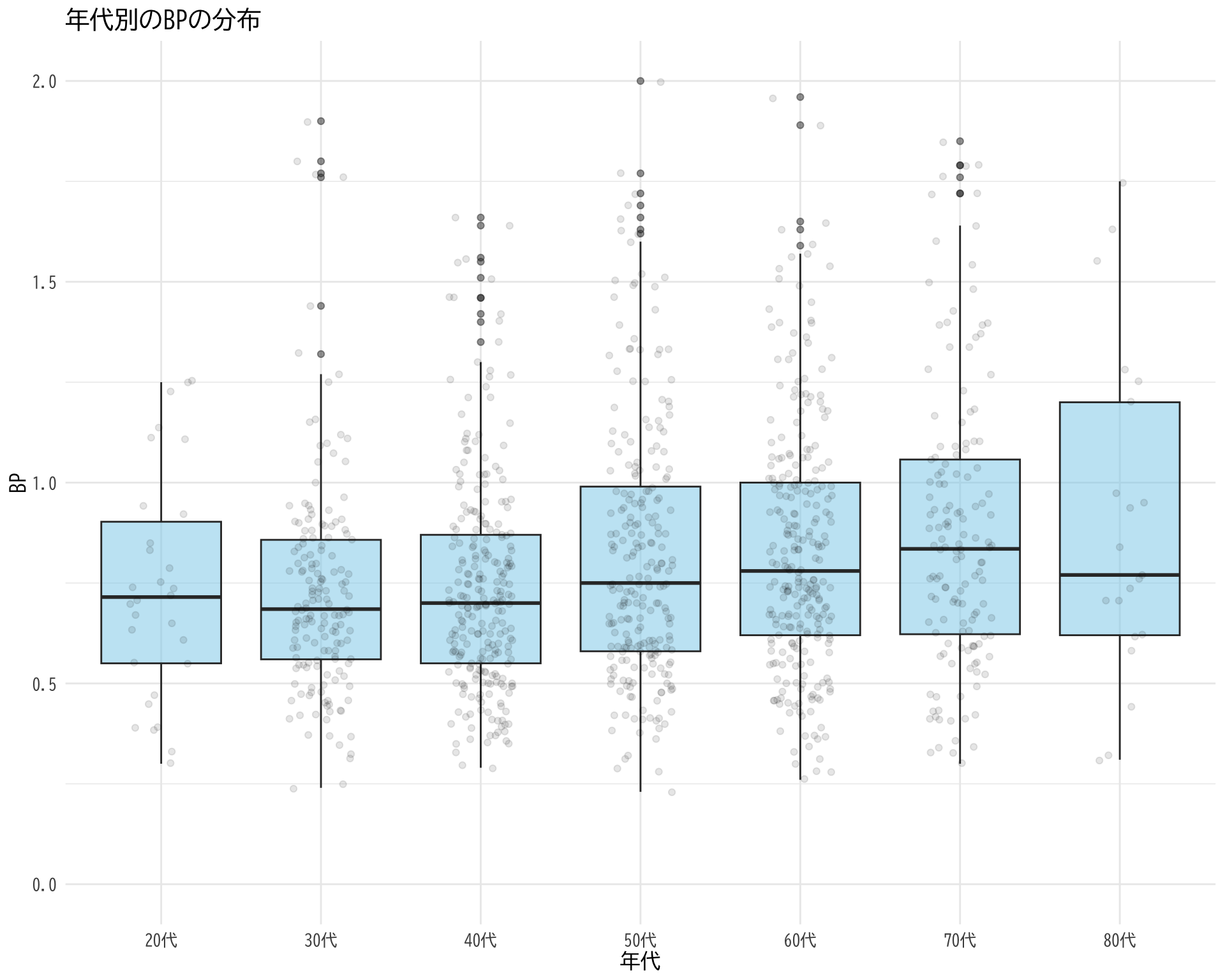
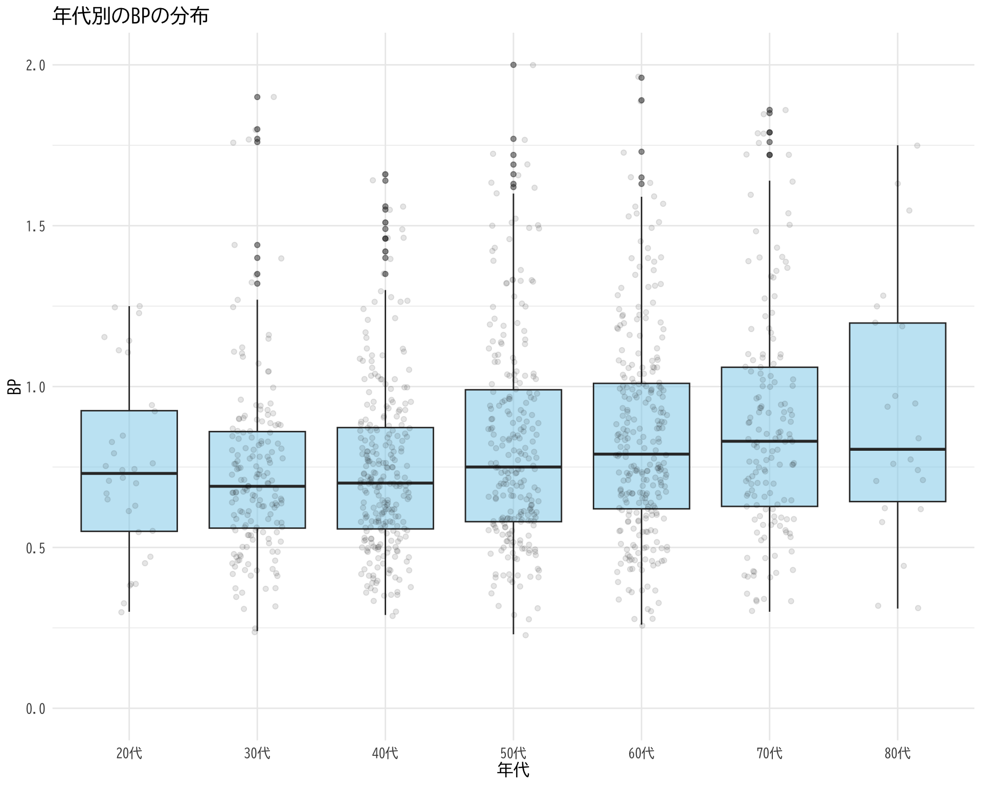
年代ごとの BP
tapply (df$ BP[df$ BP_A_flag == 0 ], df$ 年代[df$ BP_A_flag == 0 ], summary)
$`20代`
   Min. 1st Qu.  Median    Mean 3rd Qu.    Max.
 0.3000  0.5500  0.7150  0.7383  0.9025  1.2500

$`30代`
   Min. 1st Qu.  Median    Mean 3rd Qu.    Max.    NA's
 0.2400  0.5600  0.6900  0.7488  0.8600  2.2700       1

$`40代`
   Min. 1st Qu.  Median    Mean 3rd Qu.    Max.
 0.2900  0.5500  0.7000  0.7786  0.8800  4.2600

$`50代`
   Min. 1st Qu.  Median    Mean 3rd Qu.    Max.    NA's
 0.2300  0.5800  0.7550  0.8403  1.0125  2.5600       2

$`60代`
   Min. 1st Qu.  Median    Mean 3rd Qu.    Max.    NA's
 0.2600  0.6200  0.8000  0.8788  1.0300  2.7800       1

$`70代`
   Min. 1st Qu.  Median    Mean 3rd Qu.    Max.    NA's
 0.3000  0.6250  0.8400  0.8859  1.0600  2.0700       3

$`80代`
   Min. 1st Qu.  Median    Mean 3rd Qu.    Max.    NA's
 0.3100  0.6200  0.7700  0.9019  1.2000  1.7500       1
# データの準備 <- data.frame (= df$ 年代[df$ BP_A_flag == 0 ],BP = df$ BP[df$ BP_A_flag == 0 ]# ggplotでプロット ggplot (judge_by_age, aes (x = 年代, y = BP)) + # 箱ひげ図 geom_boxplot (fill = "skyblue" , alpha = 0.5 ) + # 個々のデータポイント(透明度を設定して重なりを表現) geom_jitter (width = 0.2 , alpha = 0.1 ) + theme_minimal () + labs (title = "年代別のBPの分布" ,x = "年代" ,y = "BP" ) + theme (text = element_text (family = "BIZUDGothic-Regular" , size = 12 ),# axis.text = element_text(size = 34), # axis.title = element_text(size = 45), # title = element_text(size = 45) + scale_y_continuous (limits = c (0 , 2 ))
Warning: Removed 26 rows containing non-finite values (`stat_boxplot()`).
Warning: Removed 26 rows containing missing values (`geom_point()`).
# ggsave("BP_age_dist.png", bg="white")
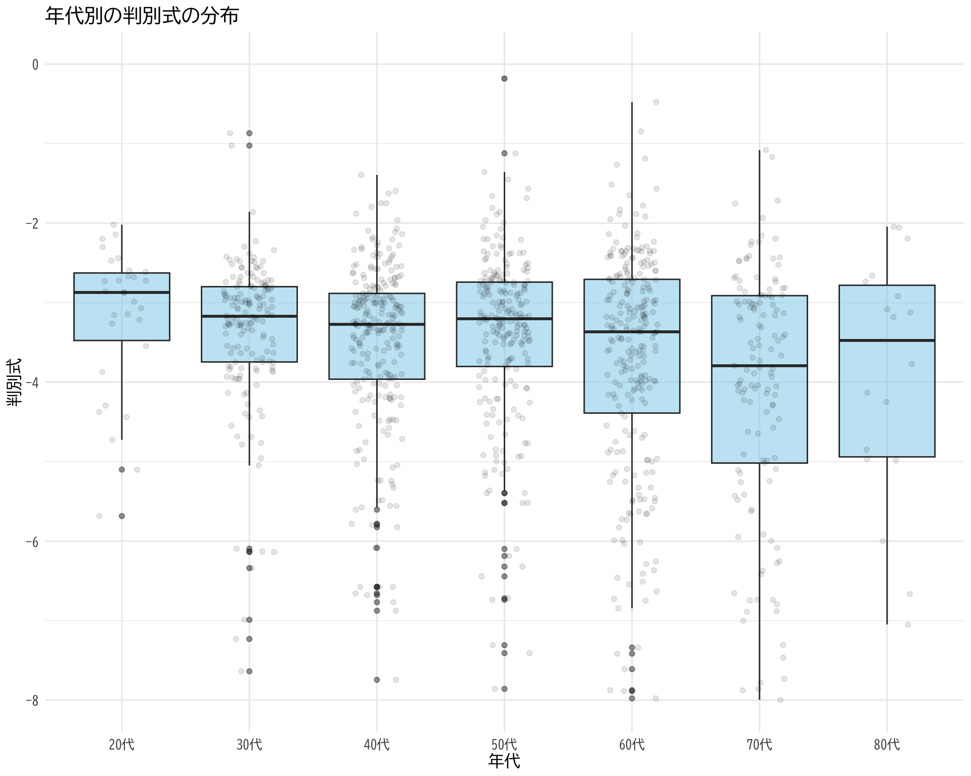
tapply (df$ 判別式[df$ BP_A_flag == 0 ], df$ 年代[df$ BP_A_flag == 0 ], summary)
$`20代`
   Min. 1st Qu.  Median    Mean 3rd Qu.    Max.
 -5.685  -3.476  -2.872  -3.193  -2.627  -2.020

$`30代`
   Min. 1st Qu.  Median    Mean 3rd Qu.    Max.    NA's
-10.675  -3.751  -3.180  -3.440  -2.803  -0.869       1

$`40代`
   Min. 1st Qu.  Median    Mean 3rd Qu.    Max.
-19.397  -3.994  -3.273  -3.551  -2.848   3.120

$`50代`
   Min. 1st Qu.  Median    Mean 3rd Qu.    Max.    NA's
-19.503  -3.931  -3.229  -3.597  -2.745  -0.182       2

$`60代`
   Min. 1st Qu.  Median    Mean 3rd Qu.    Max.    NA's
-51.117  -4.887  -3.467  -4.503  -2.738  -0.478       1

$`70代`
   Min. 1st Qu.  Median    Mean 3rd Qu.    Max.    NA's
-14.915  -5.455  -3.891  -4.530  -2.988  -1.081       3

$`80代`
   Min. 1st Qu.  Median    Mean 3rd Qu.    Max.    NA's
-70.246  -5.998  -4.131  -8.125  -2.919  -2.045       1
# データの準備 <- data.frame (= df$ 年代[df$ BP_A_flag == 0 ],= df$ 判別式[df$ BP_A_flag == 0 ]# ggplotでプロット ggplot (judge_by_age, aes (x = 年代, y = 判別式)) + # 箱ひげ図 geom_boxplot (fill = "skyblue" , alpha = 0.5 ) + # 個々のデータポイント(透明度を設定して重なりを表現) geom_jitter (width = 0.2 , alpha = 0.1 ) + theme_minimal () + labs (title = "年代別の判別式の分布" ,x = "年代" ,y = "判別式" ) + theme (text = element_text (family = "BIZUDGothic-Regular" , size = 12 ),# axis.text = element_text(size = 34), # axis.title = element_text(size = 45), # title = element_text(size = 45) + scale_y_continuous (limits = c (- 8 , 0 ))
Warning: Removed 48 rows containing non-finite values (`stat_boxplot()`).
Warning: Removed 48 rows containing missing values (`geom_point()`).
# ggsave("D_age_dist.png", bg="white")
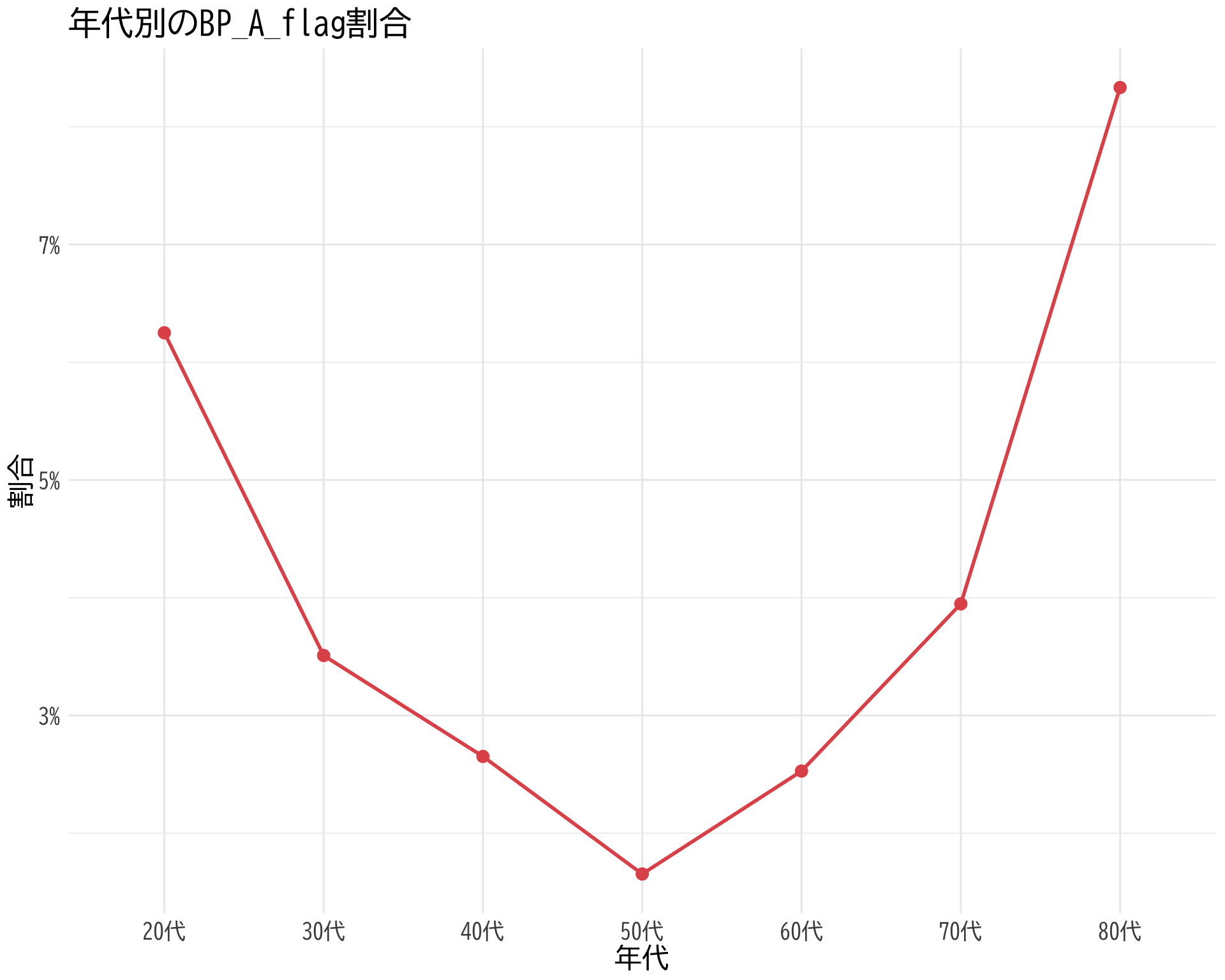
A Flag を取り除かないと結構違う
逆に 80 代以上の方が A Flag が多い.他のFlagもそうで,30代以下は圧倒的にflagが少ない.本データで平均をとればわかる.
tapply (df$ BP_A_flag, df$ 年代, summary)
$`20代`
   Min. 1st Qu.  Median    Mean 3rd Qu.    Max.
 0.0000  0.0000  0.0000  0.0625  0.0000  1.0000

$`30代`
   Min. 1st Qu.  Median    Mean 3rd Qu.    Max.
0.00000 0.00000 0.00000 0.03509 0.00000 1.00000

$`40代`
   Min. 1st Qu.  Median    Mean 3rd Qu.    Max.
0.00000 0.00000 0.00000 0.02652 0.00000 1.00000

$`50代`
   Min. 1st Qu.  Median    Mean 3rd Qu.    Max.
0.00000 0.00000 0.00000 0.01653 0.00000 1.00000

$`60代`
   Min. 1st Qu.  Median    Mean 3rd Qu.    Max.
0.00000 0.00000 0.00000 0.02527 0.00000 1.00000

$`70代`
   Min. 1st Qu.  Median    Mean 3rd Qu.    Max.
0.00000 0.00000 0.00000 0.03947 0.00000 1.00000

$`80代`
   Min. 1st Qu.  Median    Mean 3rd Qu.    Max.
0.00000 0.00000 0.00000 0.08333 0.00000 1.00000
tapply (df$ BP_A_flag, df$ 年代, function (x) sum (x, na.rm = TRUE ) / length (x))
      20代       30代       40代       50代       60代       70代       80代
0.06250000 0.03508772 0.02651515 0.01652893 0.02527076 0.03947368 0.08333333
library (ggplot2)# 割合の計算と同時にデータフレーム化 <- data.frame (= names (tapply (df$ BP_A_flag, df$ 年代, function (x) sum (x, na.rm = TRUE ) / length (x))),= as.numeric (tapply (df$ BP_A_flag, df$ 年代, function (x) sum (x, na.rm = TRUE ) / length (x)))# 折れ線プロット ggplot (bp_ratio_by_age, aes (x = 年代, y = 割合, group = 1 )) + geom_line (color = "#E15759" , size = 1 ) + geom_point (color = "#E15759" , size = 3 ) + theme_minimal () + labs (title = "年代別のBP_A_flag割合" ,x = "年代" ,y = "割合" ) + theme (text = element_text (family = "BIZUDGothic-Regular" , size = 16 ),# axis.text = element_text(size = 34), # axis.title = element_text(size = 45), # title = element_text(size = 45) + scale_y_continuous (labels = scales:: percent) # y軸をパーセント表示に
Warning: Using `size` aesthetic for lines was deprecated in ggplot2 3.4.0.
ℹ Please use `linewidth` instead.
# ggsave("portion_A_age.png", bg="white")
# データの準備 <- data.frame (= df$ 年代,BP = df$ BP# ggplotでプロット ggplot (judge_by_age, aes (x = 年代, y = BP)) + # 箱ひげ図 geom_boxplot (fill = "skyblue" , alpha = 0.5 ) + # 個々のデータポイント(透明度を設定して重なりを表現) geom_jitter (width = 0.2 , alpha = 0.1 ) + theme_minimal () + labs (title = "年代別のBPの分布" ,x = "年代" ,y = "BP" ) + theme (text = element_text (family = "BIZUDGothic-Regular" , size = 12 )+ scale_y_continuous (limits = c (0 , 2 ))
Warning: Removed 29 rows containing non-finite values (`stat_boxplot()`).
Warning: Removed 29 rows containing missing values (`geom_point()`).
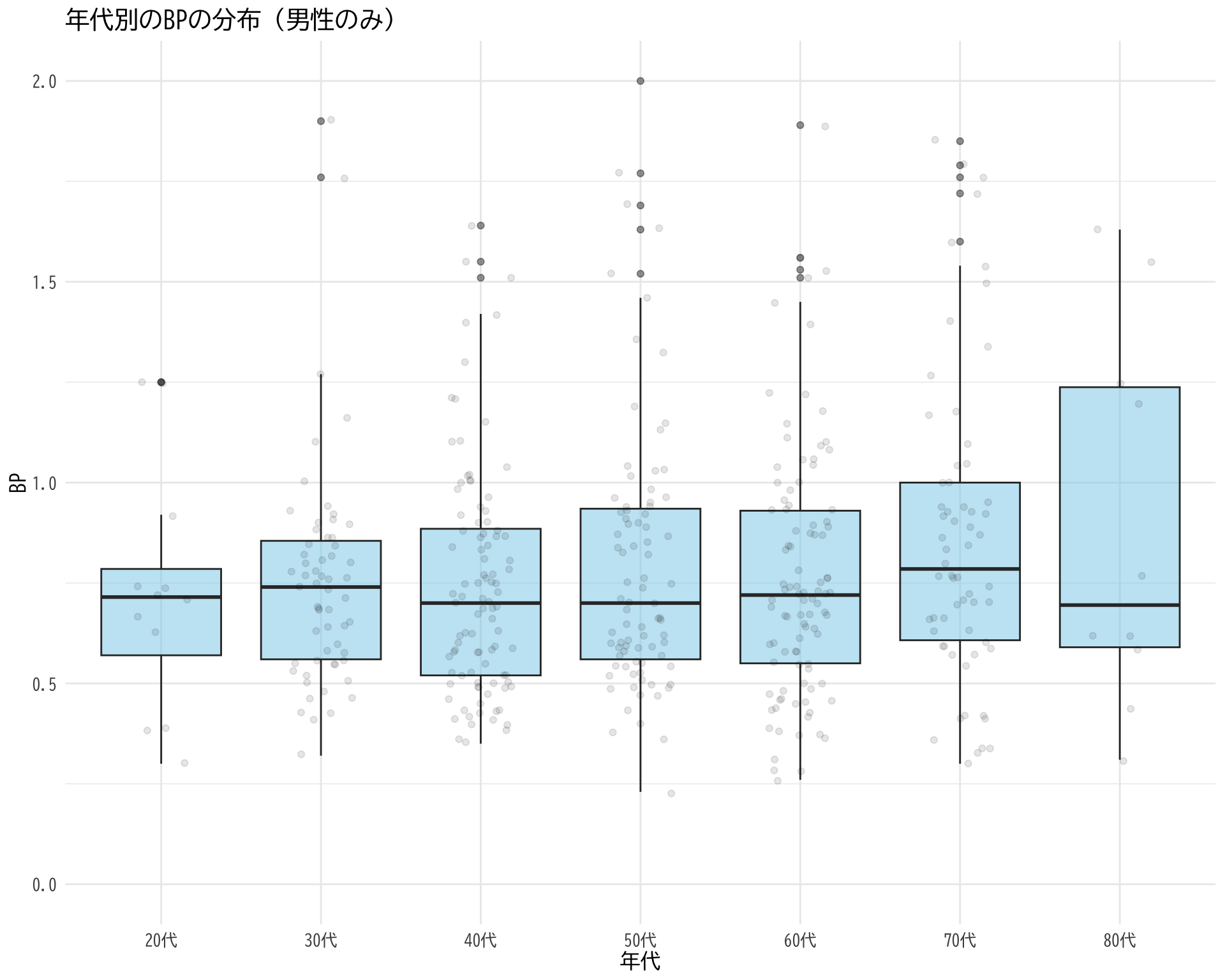
性別で制限して年代プロット
# データの準備(BP_A_flag = 0 かつ 性別 = 1 の行のみ選択) <- data.frame (= df$ 年代[df$ BP_A_flag == 0 & df$ 性別 == 1 ],BP = df$ BP[df$ BP_A_flag == 0 & df$ 性別 == 1 ]# ggplotでプロット ggplot (judge_by_age_male, aes (x = 年代, y = BP)) + # 箱ひげ図 geom_boxplot (fill = "skyblue" , alpha = 0.5 ) + # 個々のデータポイント(透明度を設定して重なりを表現) geom_jitter (width = 0.2 , alpha = 0.1 ) + theme_minimal () + labs (title = "年代別のBPの分布(男性のみ)" ,x = "年代" ,y = "BP" ) + theme (text = element_text (family = "BIZUDGothic-Regular" , size = 12 )+ scale_y_continuous (limits = c (0 ,2 ))
Warning: Removed 13 rows containing non-finite values (`stat_boxplot()`).
Warning: Removed 14 rows containing missing values (`geom_point()`).
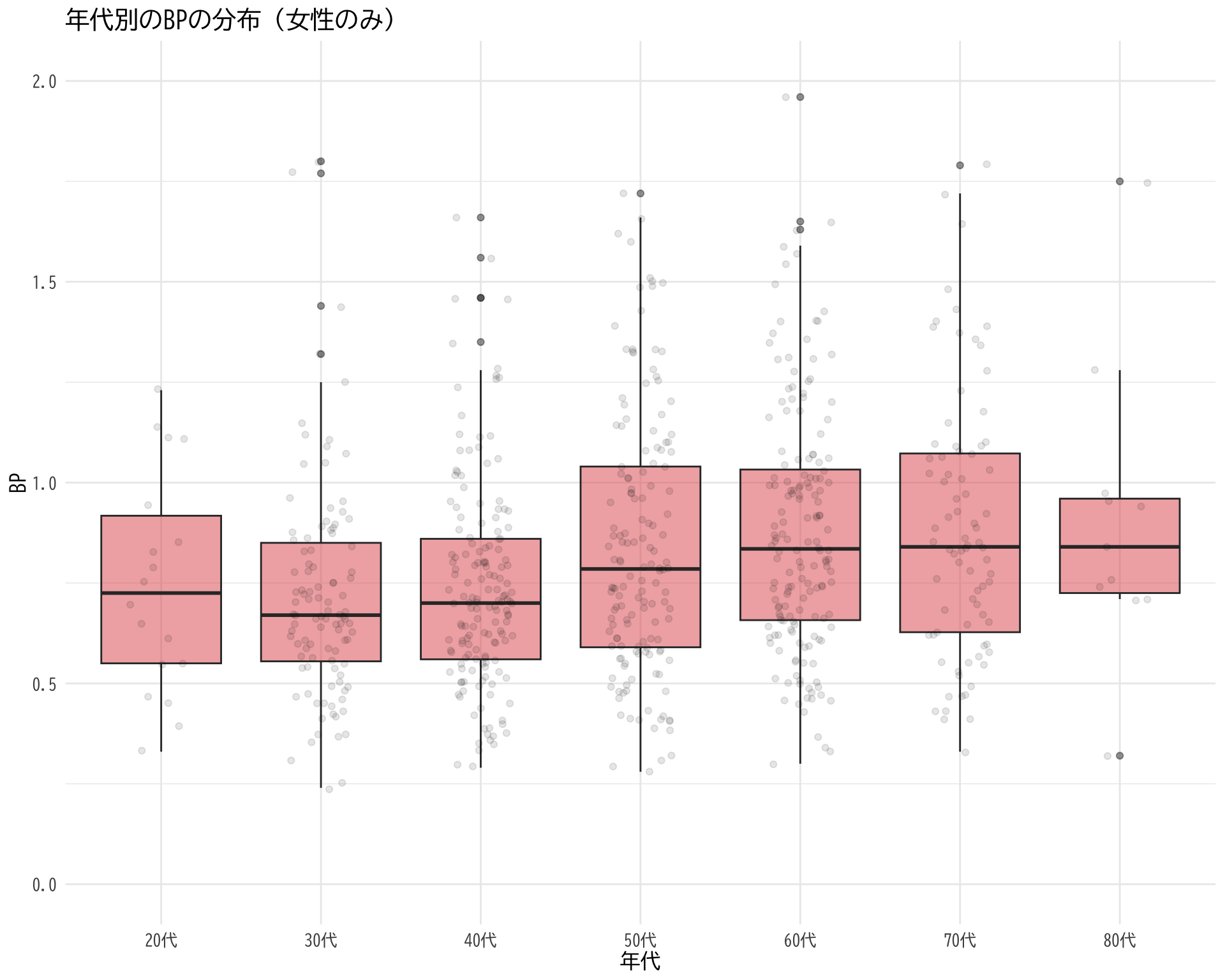
# データの準備(BP_A_flag = 0 かつ 性別 = 1 の行のみ選択) <- data.frame (= df$ 年代[df$ BP_A_flag == 0 & df$ 性別 == 2 ],BP = df$ BP[df$ BP_A_flag == 0 & df$ 性別 == 2 ]# ggplotでプロット ggplot (judge_by_age_male, aes (x = 年代, y = BP)) + # 箱ひげ図 geom_boxplot (fill = "#E15759" , alpha = 0.5 ) + # 個々のデータポイント(透明度を設定して重なりを表現) geom_jitter (width = 0.2 , alpha = 0.1 ) + theme_minimal () + labs (title = "年代別のBPの分布(女性のみ)" ,x = "年代" ,y = "BP" ) + theme (text = element_text (family = "BIZUDGothic-Regular" , size = 12 )+ scale_y_continuous (limits = c (0 ,2 ))
Warning: Removed 13 rows containing non-finite values (`stat_boxplot()`).
Warning: Removed 13 rows containing missing values (`geom_point()`).
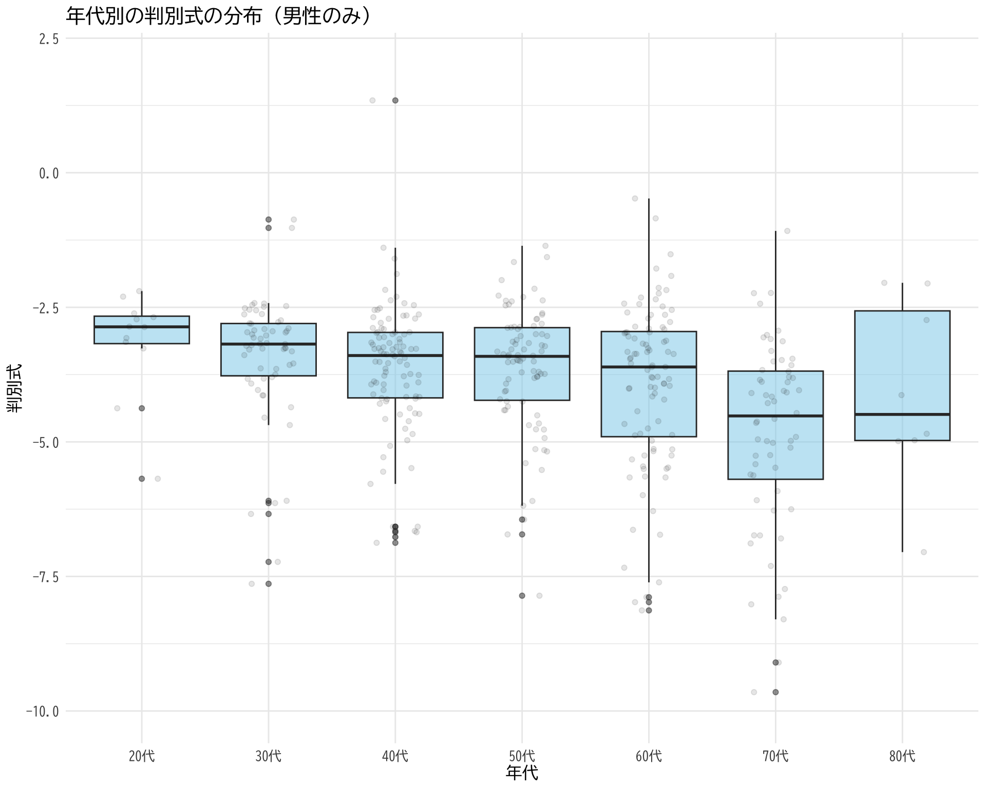
# データの準備(BP_A_flag = 0 かつ 性別 = 1 の行のみ選択) <- data.frame (= df$ 年代[df$ BP_A_flag == 0 & df$ 性別 == 1 ],= df$ 判別式[df$ BP_A_flag == 0 & df$ 性別 == 1 ]# ggplotでプロット ggplot (judge_by_age_male, aes (x = 年代, y = 判別式)) + # 箱ひげ図 geom_boxplot (fill = "skyblue" , alpha = 0.5 ) + # 個々のデータポイント(透明度を設定して重なりを表現) geom_jitter (width = 0.2 , alpha = 0.1 ) + theme_minimal () + labs (title = "年代別の判別式の分布(男性のみ)" ,x = "年代" ,y = "判別式" ) + theme (text = element_text (family = "BIZUDGothic-Regular" , size = 12 )+ scale_y_continuous (limits = c (- 10 , 2 ))
Warning: Removed 20 rows containing non-finite values (`stat_boxplot()`).
Warning: Removed 20 rows containing missing values (`geom_point()`).
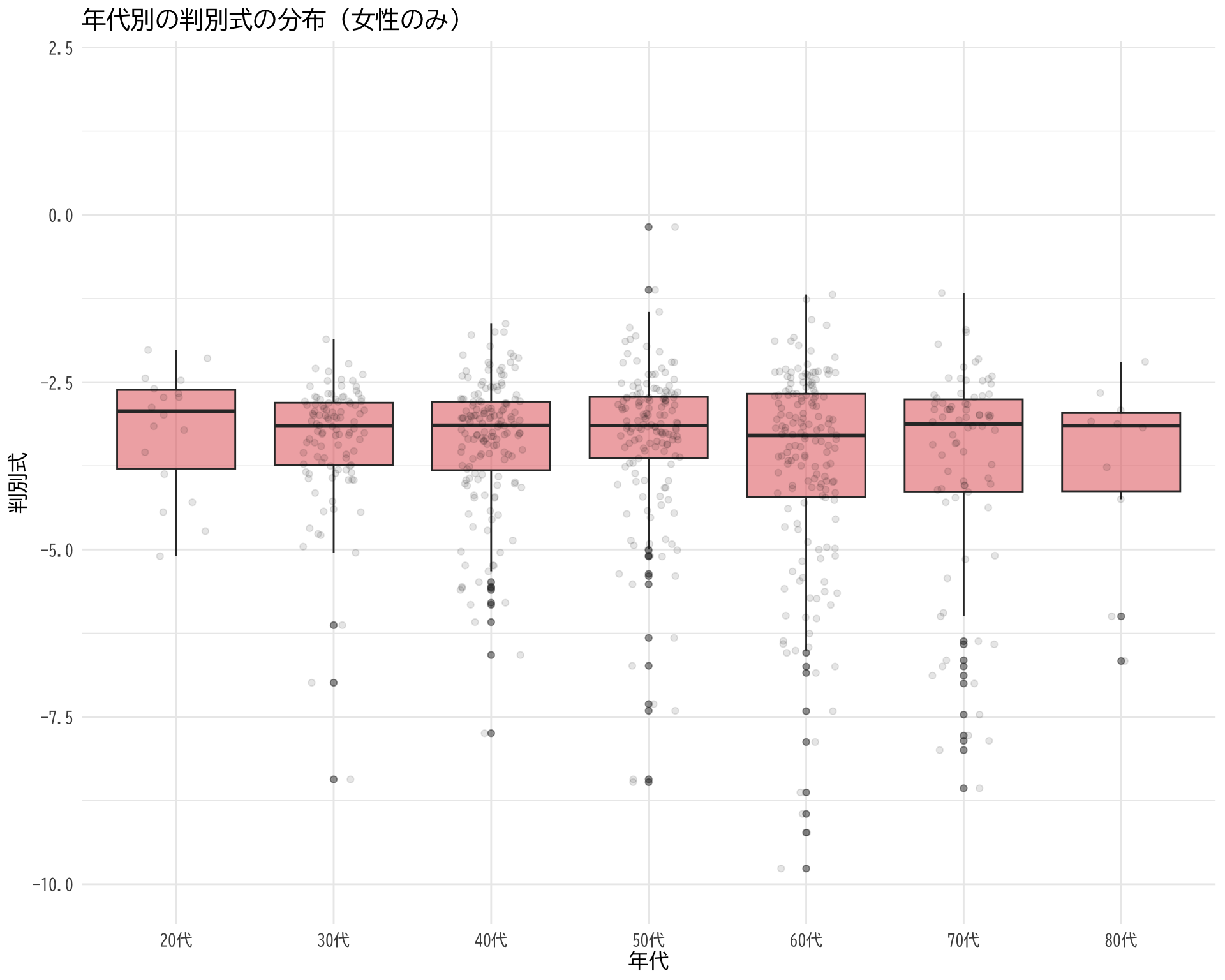
# データの準備(BP_A_flag = 0 かつ 性別 = 1 の行のみ選択) <- data.frame (= df$ 年代[df$ BP_A_flag == 0 & df$ 性別 == 2 ],= df$ 判別式[df$ BP_A_flag == 0 & df$ 性別 == 2 ]# ggplotでプロット ggplot (judge_by_age_male, aes (x = 年代, y = 判別式)) + # 箱ひげ図 geom_boxplot (fill = "#E15759" , alpha = 0.5 ) + # 個々のデータポイント(透明度を設定して重なりを表現) geom_jitter (width = 0.2 , alpha = 0.1 ) + theme_minimal () + labs (title = "年代別の判別式の分布(女性のみ)" ,x = "年代" ,y = "判別式" ) + theme (text = element_text (family = "BIZUDGothic-Regular" , size = 12 )+ scale_y_continuous (limits = c (- 10 , 2 ))
Warning: Removed 14 rows containing non-finite values (`stat_boxplot()`).
Warning: Removed 14 rows containing missing values (`geom_point()`).
性別ごとの判別式
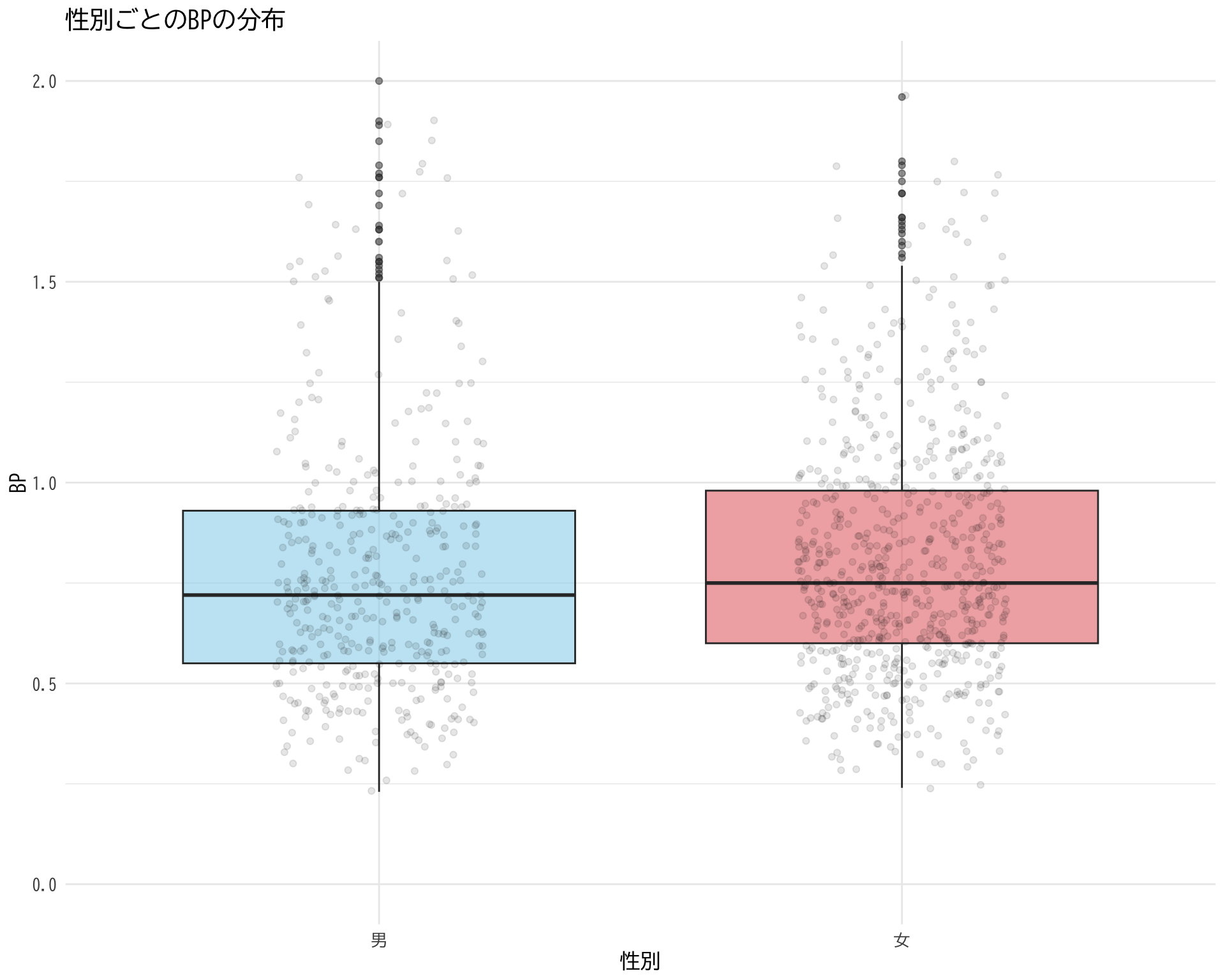
# データの準備(BP_A_flag = 0 の行のみ選択) <- data.frame (= factor (df$ 性別[df$ BP_A_flag == 0 ], levels = c (1 , 2 ), labels = c ("男" , "女" )),BP = df$ BP[df$ BP_A_flag == 0 ]# ggplotでプロット ggplot (judge_by_sex, aes (x = 性別, y = BP, fill = 性別)) + # fill = 性別 を追加 geom_boxplot (alpha = 0.5 ) + geom_jitter (width = 0.2 , alpha = 0.1 ) + theme_minimal () + labs (title = "性別ごとのBPの分布" ,x = "性別" ,y = "BP" ) + theme (text = element_text (family = "BIZUDGothic-Regular" , size = 12 ),legend.position = "none" # 凡例を非表示(色分けが明らかなため) + scale_y_continuous (limits = c (0 , 2 )) + scale_fill_manual (values = c ("男" = "skyblue" , "女" = "#E15759" )) # 性別ごとの色を指定
Warning: Removed 26 rows containing non-finite values (`stat_boxplot()`).
Warning: Removed 27 rows containing missing values (`geom_point()`).
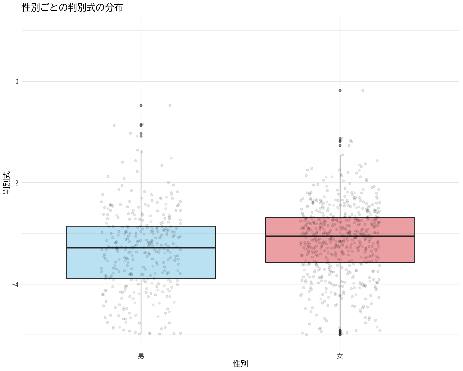
# データの準備(BP_A_flag = 0 の行のみ選択) <- data.frame (= factor (df$ 性別[df$ BP_A_flag == 0 ], levels = c (1 , 2 ), labels = c ("男" , "女" )),= df$ 判別式[df$ BP_A_flag == 0 ]# ggplotでプロット ggplot (judge_by_sex, aes (x = 性別, y = 判別式, fill = 性別)) + # fill = 性別 を追加 geom_boxplot (alpha = 0.5 ) + geom_jitter (width = 0.2 , alpha = 0.1 ) + theme_minimal () + labs (title = "性別ごとの判別式の分布" ,x = "性別" ,y = "判別式" ) + theme (text = element_text (family = "BIZUDGothic-Regular" , size = 12 ),legend.position = "none" # 凡例を非表示(色分けが明らかなため) + scale_y_continuous (limits = c (- 5 , 1 )) + scale_fill_manual (values = c ("男" = "skyblue" , "女" = "#E15759" )) # 性別ごとの色を指定
Warning: Removed 188 rows containing non-finite values (`stat_boxplot()`).
Warning: Removed 189 rows containing missing values (`geom_point()`).
体重
Warning: Removed 3 rows containing non-finite values (`stat_boxplot()`).
Warning: Removed 3 rows containing missing values (`geom_point()`).
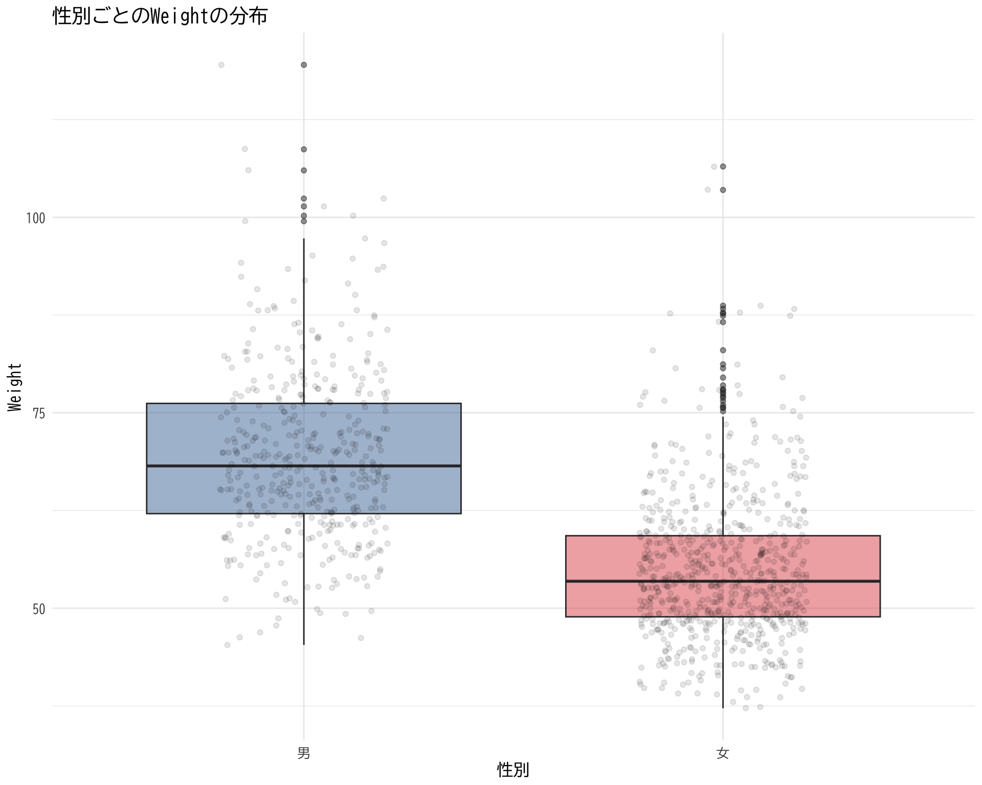
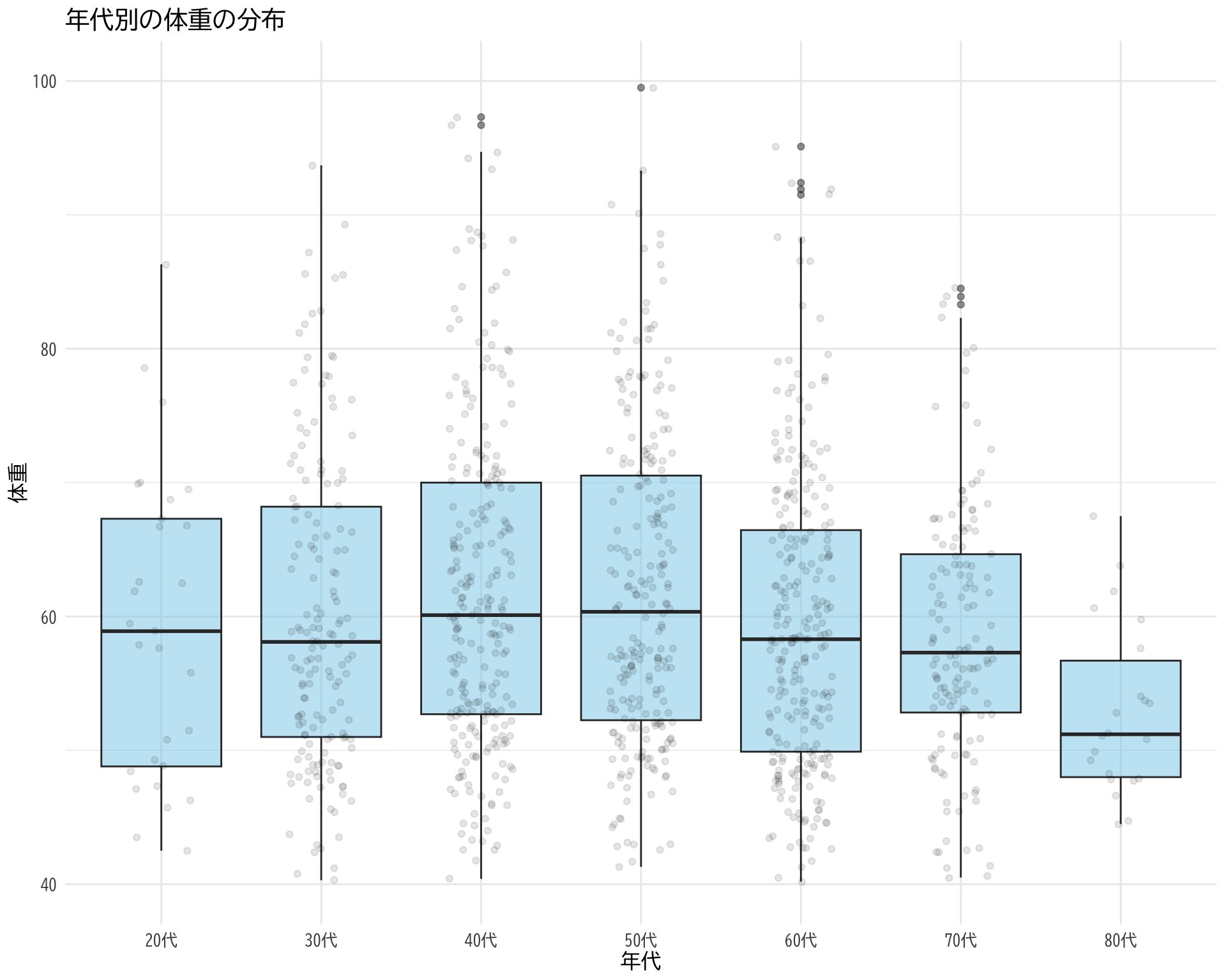
# データの準備 <- data.frame (= df$ 年代[df$ BP_A_flag == 0 ],Weight = df$ Weight[df$ BP_A_flag == 0 ]# ggplotでプロット ggplot (judge_by_age, aes (x = 年代, y = Weight)) + # 箱ひげ図 geom_boxplot (fill = "skyblue" , alpha = 0.5 ) + # 個々のデータポイント(透明度を設定して重なりを表現) geom_jitter (width = 0.2 , alpha = 0.1 ) + theme_minimal () + labs (title = "年代別の体重の分布" ,x = "年代" ,y = "体重" ) + theme (text = element_text (family = "BIZUDGothic-Regular" , size = 12 )+ scale_y_continuous (limits = c (40 , 100 ))
Warning: Removed 24 rows containing non-finite values (`stat_boxplot()`).
Warning: Removed 24 rows containing missing values (`geom_point()`).
記述で見る,BP とストレスチェックの関係
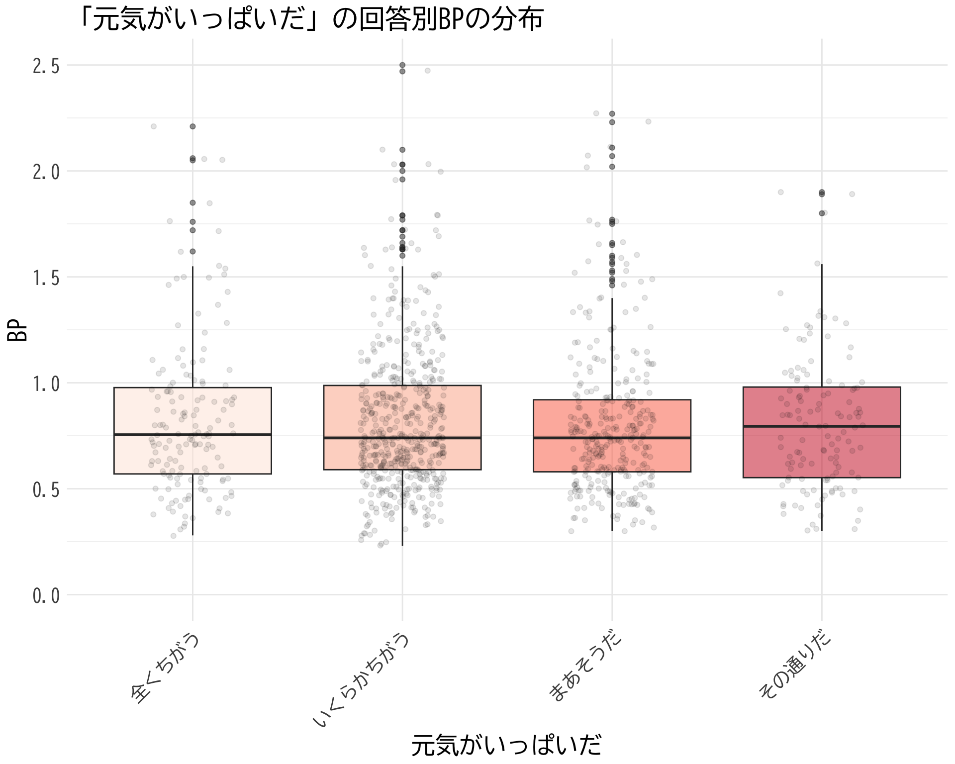
Item2「元気がいっぱいだ」
# データの準備(BP_A_flag = 0 の行のみ選択) <- data.frame (item2 = factor (df$ item2[df$ BP_A_flag == 0 ], levels = 1 : 4 ,labels = c ("全くちがう" , "いくらかちがう" , "まあそうだ" , "その通りだ" )),BP = df$ BP[df$ BP_A_flag == 0 ]# ggplotでプロット ggplot (judge_by_item2, aes (x = item2, y = BP, fill = item2)) + geom_boxplot (alpha = 0.5 ) + geom_jitter (width = 0.2 , alpha = 0.1 ) + theme_minimal () + labs (title = "「元気がいっぱいだ」の回答別BPの分布" ,x = "元気がいっぱいだ" ,y = "BP" ) + theme (text = element_text (family = "BIZUDGothic-Regular" , size = 16 ), # 基本フォントサイズを16に axis.text = element_text (size = 14 ), # 軸の目盛りの文字サイズ axis.title = element_text (size = 18 ), # 軸タイトルの文字サイズ plot.title = element_text (size = 20 ), # プロットタイトルの文字サイズ legend.position = "none" ,axis.text.x = element_text (angle = 45 , hjust = 1 )+ scale_fill_brewer (palette = "Reds" ) + scale_y_continuous (limits = c (0 , 2.5 )) # y軸の範囲を-2.5から2.5に設定
Warning: Removed 13 rows containing non-finite values (`stat_boxplot()`).
Warning: Removed 14 rows containing missing values (`geom_point()`).
\(t\) -検定でも全然棄却されない.
# データの抽出(BP_A_flag = 0 かつ item2 が 1 または 2 のデータ) <- df$ BP[df$ BP_A_flag == 0 & df$ item2 == 1 ]<- df$ BP[df$ BP_A_flag == 0 & df$ item2 == 2 ]# 等分散性の検定(Levene検定) var.test (bp_item2_1, bp_item2_2)
    F test to compare two variances

data:  bp_item2_1 and bp_item2_2
F = 1.7409, num df = 150, denom df = 522, p-value = 8.297e-06
alternative hypothesis: true ratio of variances is not equal to 1
95 percent confidence interval:
 1.358200 2.273374
sample estimates:
ratio of variances
          1.740937
# t検定の実施 t.test (bp_item2_1, bp_item2_2, var.equal = FALSE , # 等分散を仮定しない(Welchのt検定) alternative = "two.sided" ) # 両側検定
    Welch Two Sample t-test

data:  bp_item2_1 and bp_item2_2
t = 0.72118, df = 202.28, p-value = 0.4716
alternative hypothesis: true difference in means is not equal to 0
95 percent confidence interval:
 -0.05107966  0.10999245
sample estimates:
mean of x mean of y
0.8535099 0.8240535
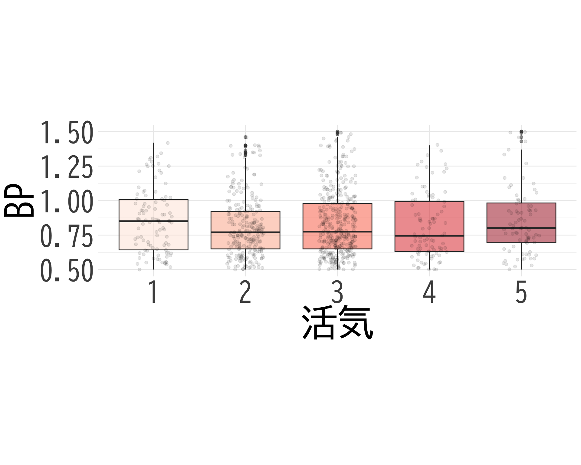
活気
# データの準備(BP_A_flag = 0 の行のみ選択) <- data.frame (= factor (df$ 活気[df$ BP_A_flag == 0 & ! is.na (df$ 活気)], levels = 1 : 5 ,labels = 1 : 5 ),BP = df$ BP[df$ BP_A_flag == 0 & ! is.na (df$ 活気)]# ggplotでプロット ggplot (judge_by_活気, aes (x = 活気, y = BP, fill = 活気)) + geom_boxplot (alpha = 0.5 ) + geom_jitter (width = 0.2 , alpha = 0.1 ) + theme_minimal () + labs (x = "活気" ,y = "BP" ) + theme (text = element_text (family = "BIZUDGothic-Regular" , size = 16 ), # 基本フォントサイズを16に axis.text = element_text (size = 34 ),axis.title = element_text (size = 45 ),legend.position = "none" + scale_fill_brewer (palette = "Reds" ) + scale_y_continuous (limits = c (0.5 , 1.5 )) + coord_fixed (ratio= 1.5 )
Warning: Removed 227 rows containing non-finite values (`stat_boxplot()`).
Warning: Removed 235 rows containing missing values (`geom_point()`).
# ggsave("活気.png", bg="white")
\(t\) -検定でも全然棄却されない.
# データの抽出(BP_A_flag = 0 かつ item2 が 1 または 2 のデータ) <- df$ BP[df$ BP_A_flag == 0 & df$ 活気 == 1 ]<- df$ BP[df$ BP_A_flag == 0 & df$ 活気 == 5 ]# 等分散性の検定(Levene検定) var.test (bp_活気_1, bp_活気_2)
    F test to compare two variances

data:  bp_活気_1 and bp_活気_2
F = 0.65652, num df = 126, denom df = 104, p-value = 0.0242
alternative hypothesis: true ratio of variances is not equal to 1
95 percent confidence interval:
 0.4524062 0.9464612
sample estimates:
ratio of variances
         0.6565195
# t検定の実施 t.test (bp_活気_1, bp_活気_2, var.equal = FALSE , # 等分散を仮定しない(Welchのt検定) alternative = "two.sided" ) # 両側検定
    Welch Two Sample t-test

data:  bp_活気_1 and bp_活気_2
t = -0.72737, df = 199.12, p-value = 0.4679
alternative hypothesis: true difference in means is not equal to 0
95 percent confidence interval:
 -0.12545032  0.05784177
sample estimates:
mean of x mean of y
0.8013386 0.8351429
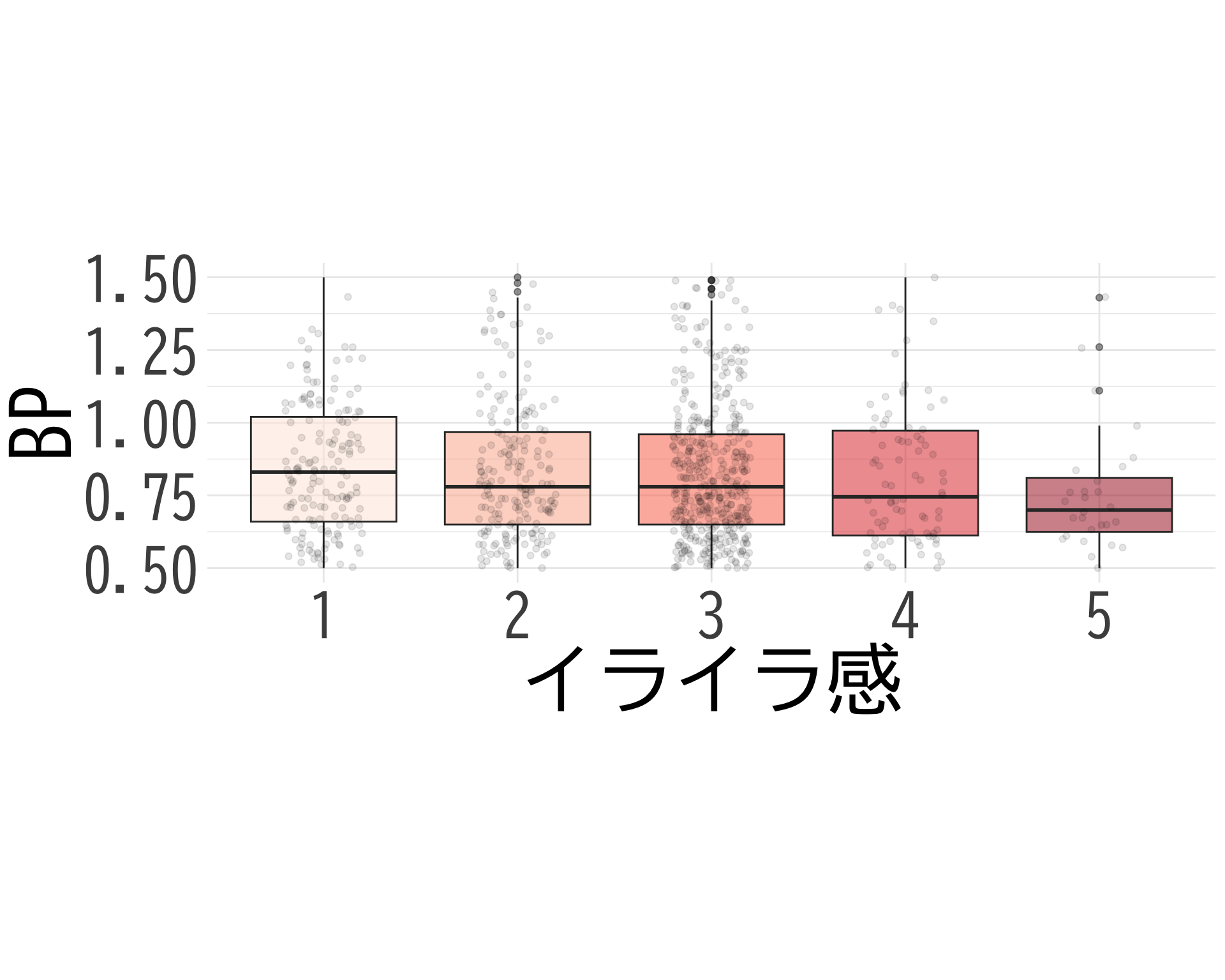
イライラ感
# データの準備(BP_A_flag = 0 の行のみ選択) <- data.frame (= factor (df$ イライラ感[df$ BP_A_flag == 0 & ! is.na (df$ イライラ感)], levels = 1 : 5 ,labels = 1 : 5 ),BP = df$ BP[df$ BP_A_flag == 0 & ! is.na (df$ イライラ感)]# ggplotでプロット ggplot (judge_by_イライラ感, aes (x = イライラ感, y = BP, fill = イライラ感)) + geom_boxplot (alpha = 0.5 ) + geom_jitter (width = 0.2 , alpha = 0.1 ) + theme_minimal () + labs (x = "イライラ感" ,y = "BP" ) + theme (text = element_text (family = "BIZUDGothic-Regular" , size = 16 ), # 基本フォントサイズを16に axis.text = element_text (size = 34 ),axis.title = element_text (size = 45 ),legend.position = "none" + scale_fill_brewer (palette = "Reds" ) + scale_y_continuous (limits = c (0.5 , 1.5 )) + # y軸の範囲を-2.5から2.5に設定 coord_fixed (ratio = 1.5 )
Warning: Removed 226 rows containing non-finite values (`stat_boxplot()`).
Warning: Removed 234 rows containing missing values (`geom_point()`).
# ggsave("イライラ感.png", bg="white")
\(t\) -検定でも全然棄却されない.
# データの抽出(BP_A_flag = 0 かつ item2 が 1 または 2 のデータ) <- df$ BP[df$ BP_A_flag == 0 & df$ イライラ感 == 1 ]<- df$ BP[df$ BP_A_flag == 0 & df$ イライラ感 == 5 ]# 等分散性の検定(Levene検定) var.test (bp_イライラ感_1, bp_イライラ感_2)
    F test to compare two variances

data:  bp_イライラ感_1 and bp_イライラ感_2
F = 0.9411, num df = 207, denom df = 32, p-value = 0.7698
alternative hypothesis: true ratio of variances is not equal to 1
95 percent confidence interval:
 0.5235379 1.5235640
sample estimates:
ratio of variances
         0.9410959
# t検定の実施 t.test (bp_イライラ感_1, bp_イライラ感_2, var.equal = FALSE , # 等分散を仮定しない(Welchのt検定) alternative = "two.sided" ) # 両側検定
    Welch Two Sample t-test

data:  bp_イライラ感_1 and bp_イライラ感_2
t = 0.67062, df = 42.124, p-value = 0.5061
alternative hypothesis: true difference in means is not equal to 0
95 percent confidence interval:
 -0.09811264  0.19578456
sample estimates:
mean of x mean of y
0.8500481 0.8012121
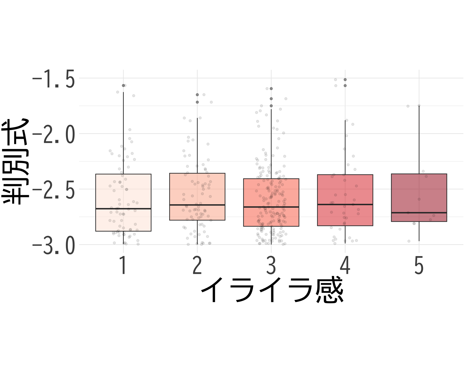
イライラ感×判別式
# データの準備(BP_A_flag = 0 の行のみ選択) <- data.frame (= factor (df$ イライラ感[df$ BP_A_flag == 0 & ! is.na (df$ イライラ感)], levels = 1 : 5 ,labels = 1 : 5 ),= df$ 判別式[df$ BP_A_flag == 0 & ! is.na (df$ イライラ感)]# ggplotでプロット ggplot (judge_by_イライラ感, aes (x = イライラ感, y = 判別式, fill = イライラ感)) + geom_boxplot (alpha = 0.5 ) + geom_jitter (width = 0.2 , alpha = 0.1 ) + theme_minimal () + labs (x = "イライラ感" ,y = "判別式" ) + theme (text = element_text (family = "BIZUDGothic-Regular" , size = 16 ), # 基本フォントサイズを16に axis.text = element_text (size = 34 ),axis.title = element_text (size = 45 ),legend.position = "none" + scale_fill_brewer (palette = "Reds" ) + scale_y_continuous (limits = c (- 3 , - 1.5 )) + coord_fixed (ratio = 1.5 )
Warning: Removed 750 rows containing non-finite values (`stat_boxplot()`).
Warning: Removed 751 rows containing missing values (`geom_point()`).
# ggsave("イライラ感×判別式.png", bg="white")
これでも \(p\) -値が出ない.
# データの抽出(BP_A_flag = 0 かつ item2 が 1 または 2 のデータ) <- df$ 判別式[df$ BP_A_flag == 0 & df$ イライラ感 == 1 ]<- df$ 判別式[df$ BP_A_flag == 0 & df$ イライラ感 == 5 ]# 等分散性の検定(Levene検定) var.test (bp_イライラ感_1, bp_イライラ感_2)
    F test to compare two variances

data:  bp_イライラ感_1 and bp_イライラ感_2
F = 2.4249, num df = 207, denom df = 32, p-value = 0.003911
alternative hypothesis: true ratio of variances is not equal to 1
95 percent confidence interval:
 1.348961 3.925654
sample estimates:
ratio of variances
          2.424852
# t検定の実施 t.test (bp_イライラ感_1, bp_イライラ感_2, var.equal = FALSE , # 等分散を仮定しない(Welchのt検定) alternative = "two.sided" ) # 両側検定
    Welch Two Sample t-test

data:  bp_イライラ感_1 and bp_イライラ感_2
t = -1.1423, df = 59.985, p-value = 0.2579
alternative hypothesis: true difference in means is not equal to 0
95 percent confidence interval:
 -1.8859888  0.5149507
sample estimates:
mean of x mean of y
-4.386822 -3.701303
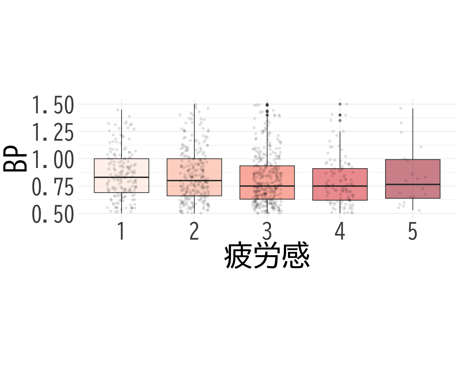
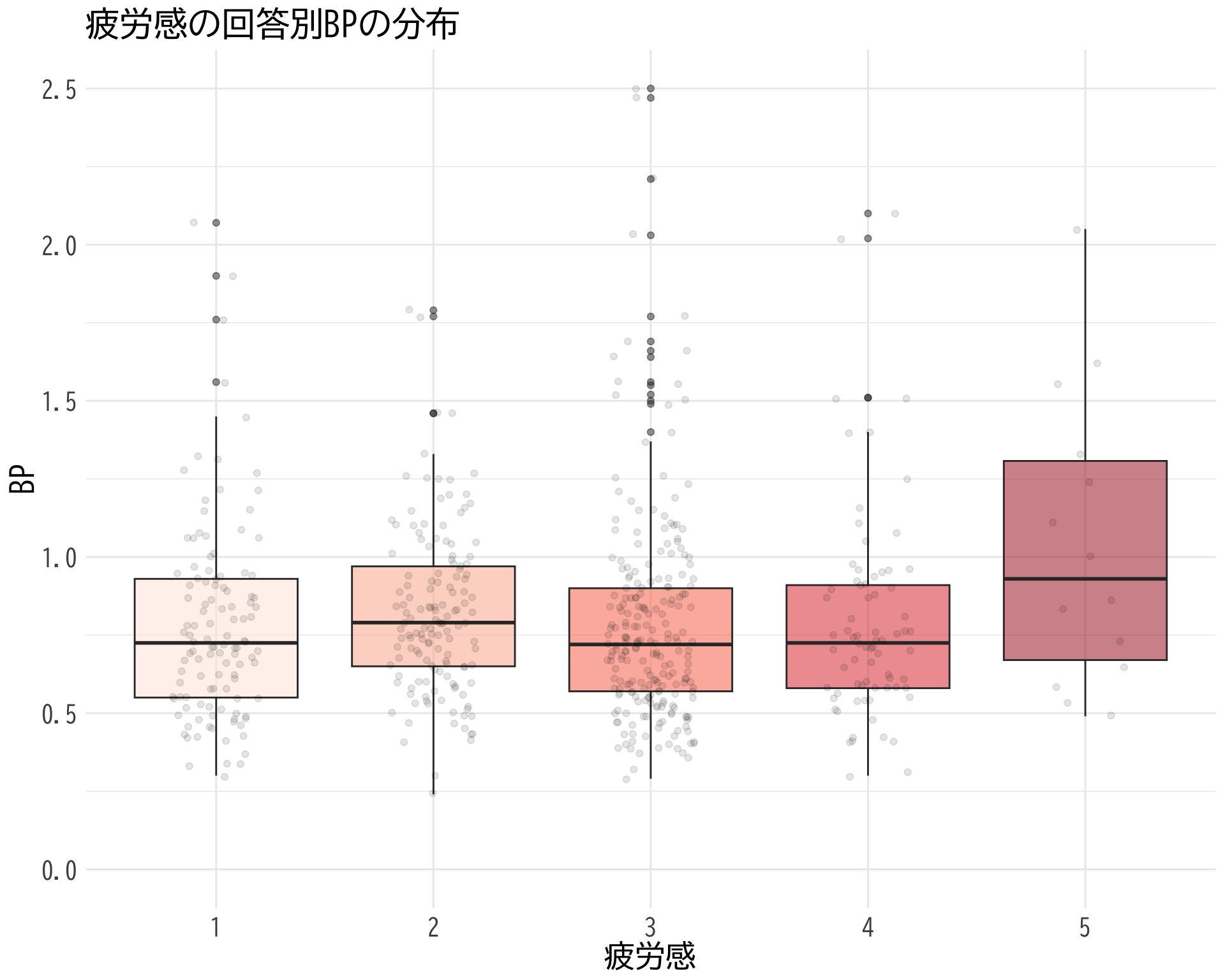
疲労感:お?
# データの準備(BP_A_flag = 0 の行のみ選択) <- data.frame (= factor (df$ 疲労感[df$ BP_A_flag == 0 & ! is.na (df$ 疲労感)], levels = 1 : 5 ,labels = 1 : 5 ),BP = df$ BP[df$ BP_A_flag == 0 & ! is.na (df$ 疲労感)]# ggplotでプロット ggplot (judge_by_疲労感, aes (x = 疲労感, y = BP, fill = 疲労感)) + geom_boxplot (alpha = 0.5 ) + geom_jitter (width = 0.2 , alpha = 0.1 ) + theme_minimal () + labs (x = "疲労感" ,y = "BP" ) + theme (text = element_text (family = "BIZUDGothic-Regular" , size = 16 ), # 基本フォントサイズを16に axis.text = element_text (size = 34 ),axis.title = element_text (size = 45 ),legend.position = "none" + scale_fill_brewer (palette = "Reds" ) + scale_y_continuous (limits = c (0.5 , 1.5 )) + coord_fixed (ratio = 1.5 )
Warning: Removed 227 rows containing non-finite values (`stat_boxplot()`).
Warning: Removed 236 rows containing missing values (`geom_point()`).
# ggsave("疲労感.png", bg="white")
# データの抽出(BP_A_flag = 0 かつ item2 が 1 または 2 のデータ) <- df$ BP[df$ BP_A_flag == 0 & df$ 疲労感 == 1 ]<- df$ BP[df$ BP_A_flag == 0 & df$ 疲労感 == 5 ]# 等分散性の検定(Levene検定) var.test (bp_疲労感_1, bp_疲労感_2)
    F test to compare two variances

data:  bp_疲労感_1 and bp_疲労感_2
F = 0.90522, num df = 221, denom df = 24, p-value = 0.68
alternative hypothesis: true ratio of variances is not equal to 1
95 percent confidence interval:
 0.4579951 1.5432604
sample estimates:
ratio of variances
         0.9052217
# t検定の実施 t.test (bp_疲労感_1, bp_疲労感_2, var.equal = FALSE , # 等分散を仮定しない(Welchのt検定) alternative = "two.sided" ) # 両側検定
    Welch Two Sample t-test

data:  bp_疲労感_1 and bp_疲労感_2
t = -1.4641, df = 29.11, p-value = 0.1539
alternative hypothesis: true difference in means is not equal to 0
95 percent confidence interval:
 -0.32693343  0.05410821
sample estimates:
mean of x mean of y
0.8323874 0.9688000
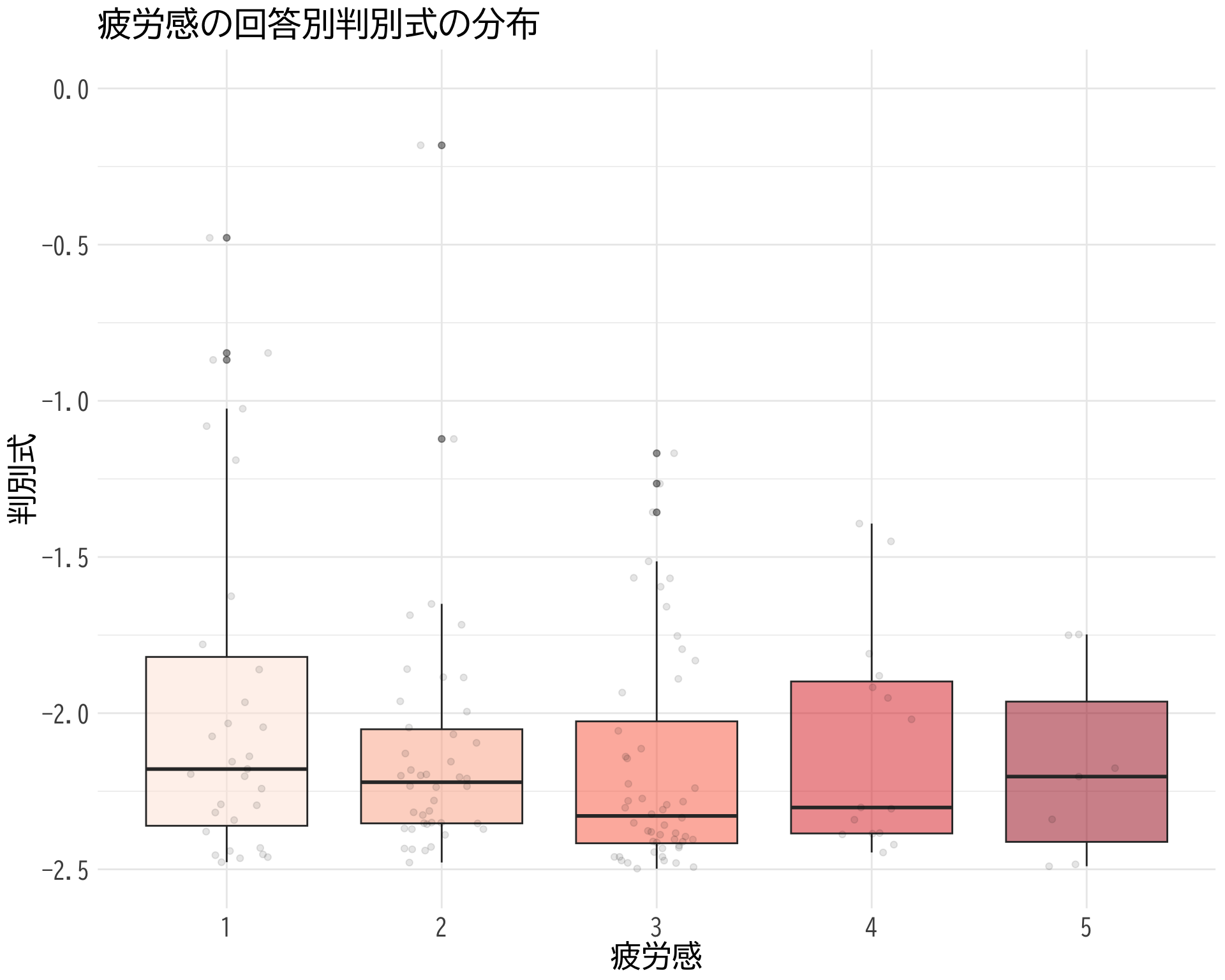
疲労感×判別式
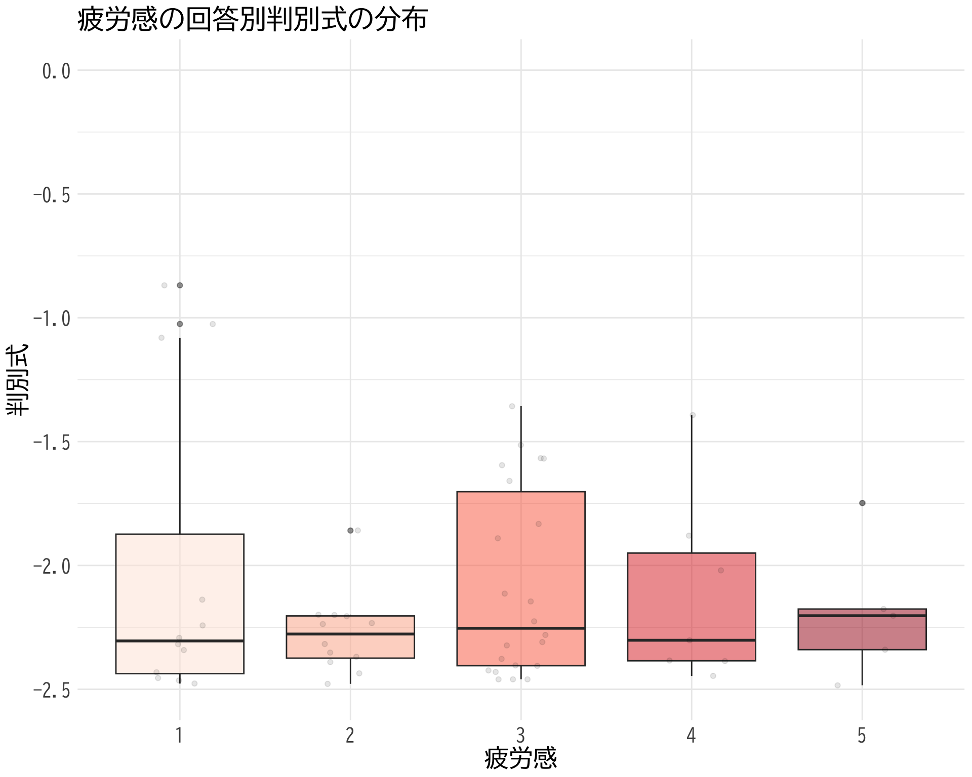
# データの準備(BP_A_flag = 0 の行のみ選択) <- data.frame (= factor (df$ 疲労感[df$ BP_A_flag == 0 & ! is.na (df$ 疲労感)], levels = 1 : 5 ,labels = 1 : 5 ),= df$ 判別式[df$ BP_A_flag == 0 & ! is.na (df$ 疲労感)]# ggplotでプロット ggplot (judge_by_疲労感, aes (x = 疲労感, y = 判別式, fill = 疲労感)) + geom_boxplot (alpha = 0.5 ) + geom_jitter (width = 0.2 , alpha = 0.1 ) + theme_minimal () + labs (title = "疲労感の回答別判別式の分布" ,x = "疲労感" ,y = "判別式" ) + theme (text = element_text (family = "BIZUDGothic-Regular" , size = 16 ), # 基本フォントサイズを16に axis.text = element_text (size = 14 ), # 軸の目盛りの文字サイズ axis.title = element_text (size = 18 ), # 軸タイトルの文字サイズ plot.title = element_text (size = 20 ), # プロットタイトルの文字サイズ legend.position = "none" + scale_fill_brewer (palette = "Reds" ) + scale_y_continuous (limits = c (- 2.5 , 0 )) # y軸の範囲を-2.5から2.5に設定
Warning: Removed 980 rows containing non-finite values (`stat_boxplot()`).
Warning: Removed 980 rows containing missing values (`geom_point()`).
これだと \(p\) -値が出なくなる.
# データの抽出(BP_A_flag = 0 かつ item2 が 1 または 2 のデータ) <- df$ 判別式[df$ BP_A_flag == 0 & df$ 疲労感 == 1 ]<- df$ 判別式[df$ BP_A_flag == 0 & df$ 疲労感 == 5 ]# 等分散性の検定(Levene検定) var.test (bp_疲労感_1, bp_疲労感_2)
    F test to compare two variances

data:  bp_疲労感_1 and bp_疲労感_2
F = 0.22275, num df = 221, denom df = 24, p-value = 1.37e-09
alternative hypothesis: true ratio of variances is not equal to 1
95 percent confidence interval:
 0.1127002 0.3797545
sample estimates:
ratio of variances
         0.2227505
# t検定の実施 t.test (bp_疲労感_1, bp_疲労感_2, var.equal = FALSE , # 等分散を仮定しない(Welchのt検定) alternative = "two.sided" ) # 両側検定
    Welch Two Sample t-test

data:  bp_疲労感_1 and bp_疲労感_2
t = 0.42617, df = 25.217, p-value = 0.6736
alternative hypothesis: true difference in means is not equal to 0
95 percent confidence interval:
 -1.344378  2.046292
sample estimates:
mean of x mean of y
-3.819243 -4.170200
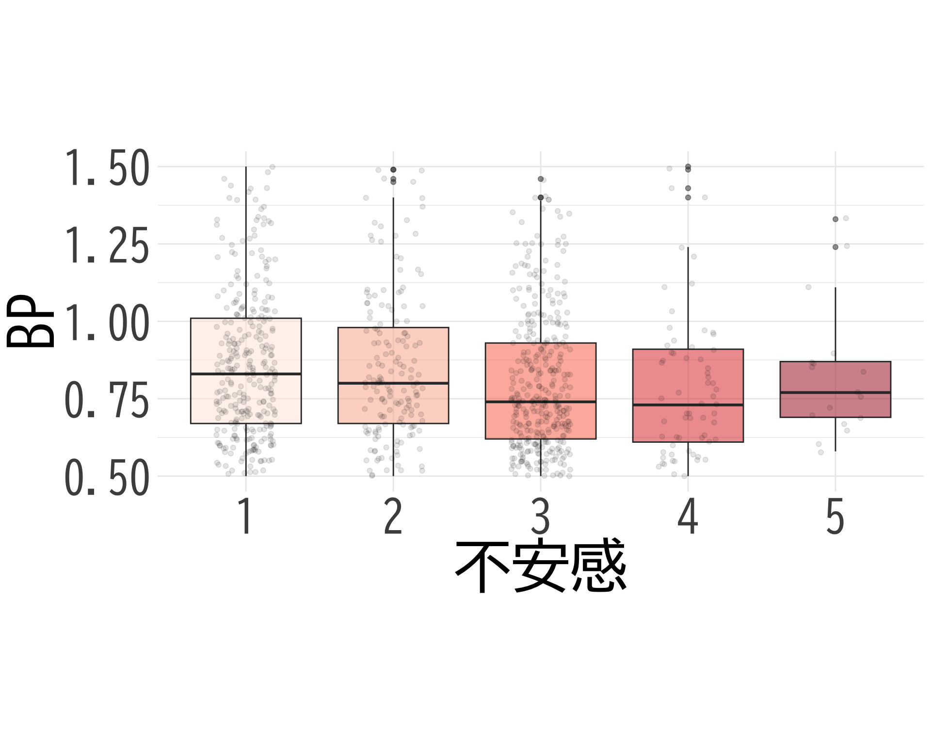
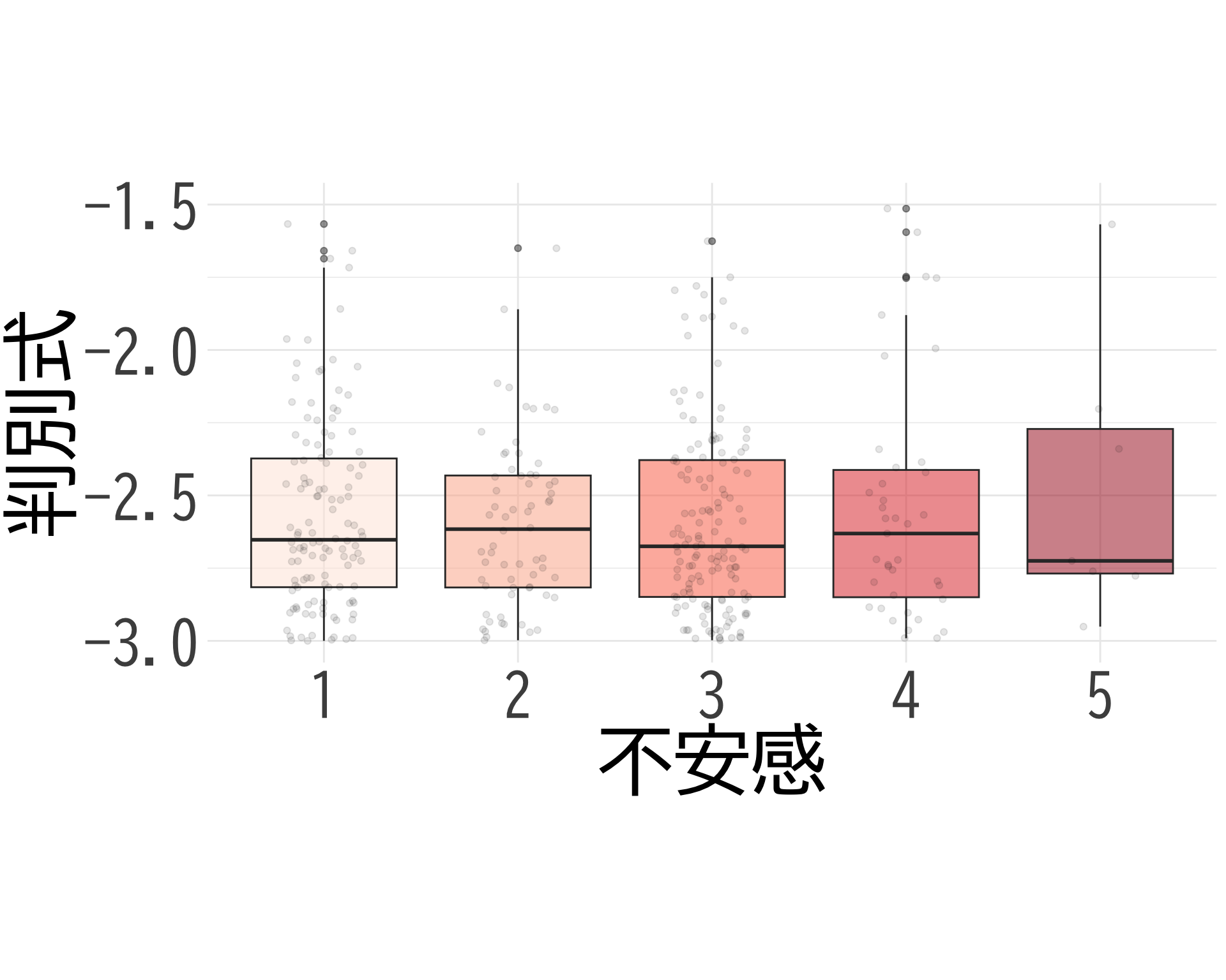
不安感:おお!?
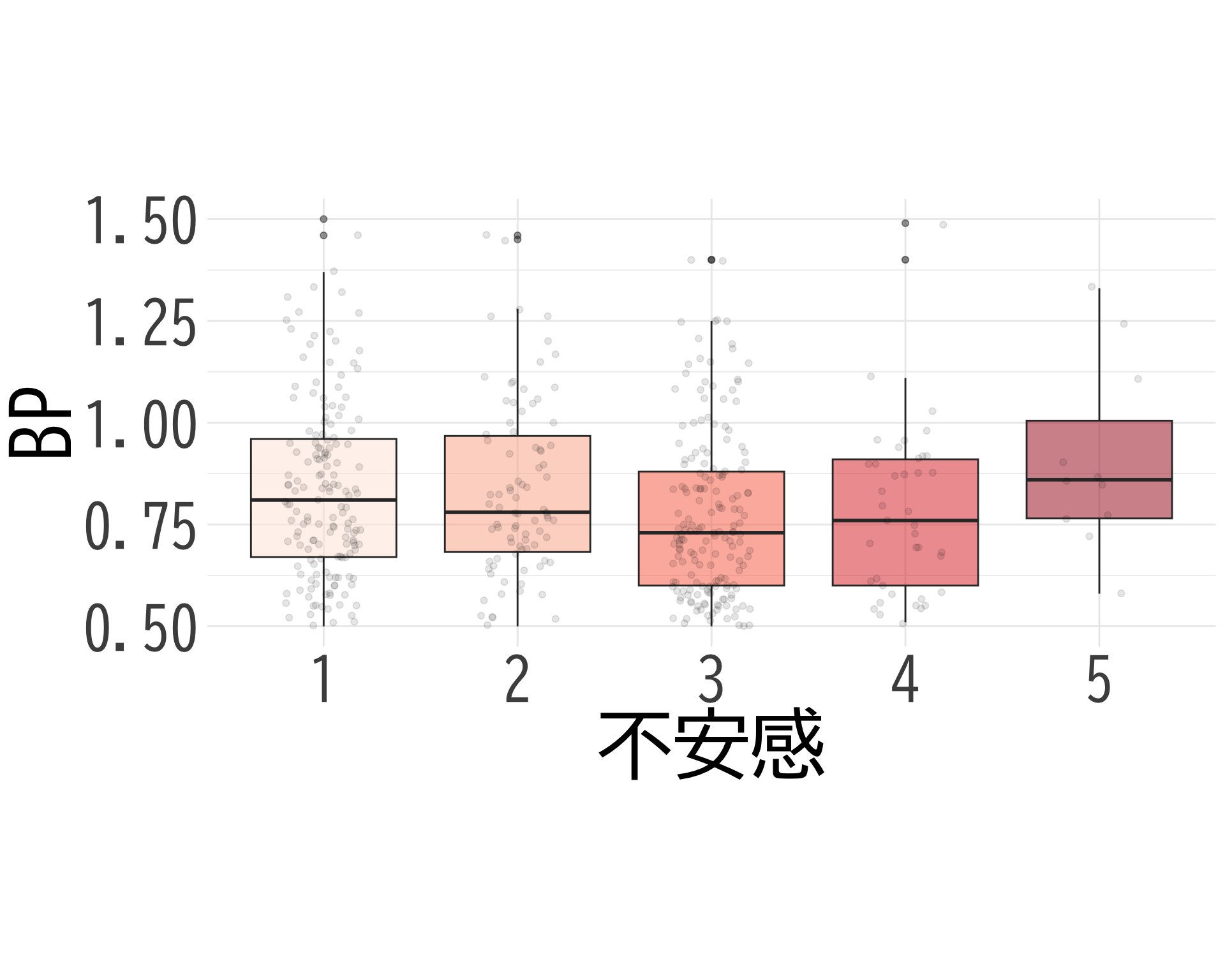
# データの準備(BP_A_flag = 0 の行のみ選択) <- data.frame (= factor (df$ 不安感[df$ BP_A_flag == 0 & ! is.na (df$ 不安感)], levels = 1 : 5 ,labels = 1 : 5 ),BP = df$ BP[df$ BP_A_flag == 0 & ! is.na (df$ 不安感)]# ggplotでプロット ggplot (judge_by_不安感, aes (x = 不安感, y = BP, fill = 不安感)) + geom_boxplot (alpha = 0.5 ) + geom_jitter (width = 0.2 , alpha = 0.1 ) + theme_minimal () + labs (x = "不安感" ,y = "BP" ) + theme (text = element_text (family = "BIZUDGothic-Regular" , size = 16 ), # 基本フォントサイズを16に axis.text = element_text (size = 34 ),axis.title = element_text (size = 45 ),legend.position = "none" + scale_fill_brewer (palette = "Reds" ) + scale_y_continuous (limits = c (0.5 , 1.5 )) + coord_fixed (ratio = 2.1 )
Warning: Removed 226 rows containing non-finite values (`stat_boxplot()`).
Warning: Removed 238 rows containing missing values (`geom_point()`).
# ggsave("不安感_備考あり.png", bg="white")
# データの抽出(BP_A_flag = 0 かつ item2 が 1 または 2 のデータ) <- df$ BP[df$ BP_A_flag == 0 & df$ 不安感 == 1 ]<- df$ BP[df$ BP_A_flag == 0 & df$ 不安感 >= 4 ]# 等分散性の検定(Levene検定) var.test (bp_不安感_1, bp_不安感_2)
    F test to compare two variances

data:  bp_不安感_1 and bp_不安感_2
F = 0.57987, num df = 375, denom df = 106, p-value = 0.0002183
alternative hypothesis: true ratio of variances is not equal to 1
95 percent confidence interval:
 0.4212997 0.7772372
sample estimates:
ratio of variances
         0.5798674
# t検定の実施 t.test (bp_不安感_1, bp_不安感_2, var.equal = FALSE , # 等分散を仮定しない(Welchのt検定) alternative = "two.sided" ) # 両側検定
    Welch Two Sample t-test

data:  bp_不安感_1 and bp_不安感_2
t = -0.56412, df = 142.77, p-value = 0.5736
alternative hypothesis: true difference in means is not equal to 0
95 percent confidence interval:
 -0.12346548  0.06864196
sample estimates:
mean of x mean of y
0.8338032 0.8612150
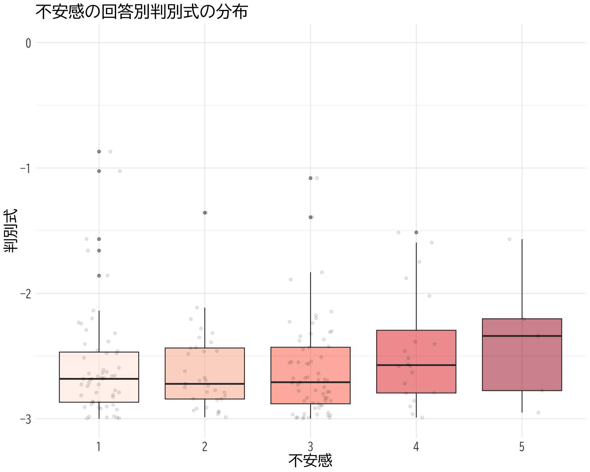
不安感×判別式
やはり判別式も有意に低いが,少し分散が大きくなる.
# データの準備(BP_A_flag = 0 の行のみ選択) <- data.frame (= factor (df$ 不安感[df$ BP_A_flag == 0 & ! is.na (df$ 不安感)], levels = 1 : 5 ,labels = 1 : 5 ),= df$ 判別式[df$ BP_A_flag == 0 & ! is.na (df$ 不安感)]# ggplotでプロット ggplot (judge_by_不安感, aes (x = 不安感, y = 判別式, fill = 不安感)) + geom_boxplot (alpha = 0.5 ) + geom_jitter (width = 0.2 , alpha = 0.1 ) + theme_minimal () + labs (x = "不安感" ,y = "判別式" ) + theme (text = element_text (family = "BIZUDGothic-Regular" , size = 16 ), # 基本フォントサイズを16に axis.text = element_text (size = 34 ),axis.title = element_text (size = 45 ),legend.position = "none" + scale_fill_brewer (palette = "Reds" ) + scale_y_continuous (limits = c (- 3 , - 1.5 )) + coord_fixed (ratio= 1.5 )
Warning: Removed 750 rows containing non-finite values (`stat_boxplot()`).
Warning: Removed 750 rows containing missing values (`geom_point()`).
# ggsave("不安感×判別式.png", bg="white")
# データの抽出(BP_A_flag = 0 かつ item2 が 1 または 2 のデータ) <- df$ 判別式[df$ BP_A_flag == 0 & df$ 不安感 == 1 ]<- df$ 判別式[df$ BP_A_flag == 0 & df$ 不安感 == 5 ]# 等分散性の検定(Levene検定) var.test (bp_不安感_1, bp_不安感_2)
    F test to compare two variances

data:  bp_不安感_1 and bp_不安感_2
F = 4.1508, num df = 375, denom df = 19, p-value = 0.0006691
alternative hypothesis: true ratio of variances is not equal to 1
95 percent confidence interval:
 1.925150 7.329238
sample estimates:
ratio of variances
          4.150766
# t検定の実施 t.test (bp_不安感_1, bp_不安感_2, var.equal = FALSE , # 等分散を仮定しない(Welchのt検定) alternative = "two.sided" ) # 両側検定
    Welch Two Sample t-test

data:  bp_不安感_1 and bp_不安感_2
t = -2.4675, df = 28.246, p-value = 0.01993
alternative hypothesis: true difference in means is not equal to 0
95 percent confidence interval:
 -1.06223073 -0.09878097
sample estimates:
mean of x mean of y
-3.868806 -3.288300
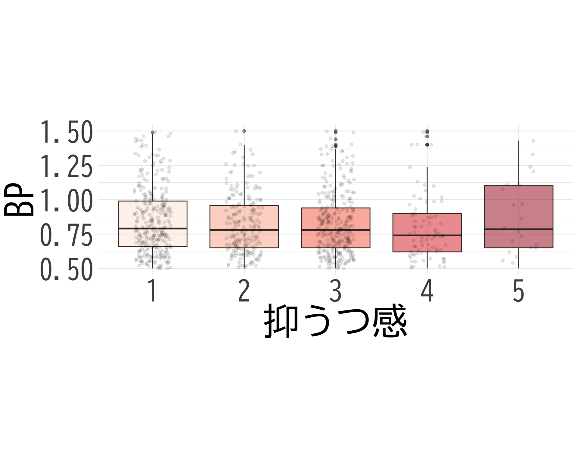
抑うつ感
# データの準備(BP_A_flag = 0 の行のみ選択) <- data.frame (= factor (df$ 抑うつ感[df$ BP_A_flag == 0 & ! is.na (df$ 抑うつ感)], levels = 1 : 5 ,labels = 1 : 5 ),BP = df$ BP[df$ BP_A_flag == 0 & ! is.na (df$ 抑うつ感)]# ggplotでプロット ggplot (judge_by_抑うつ感, aes (x = 抑うつ感, y = BP, fill = 抑うつ感)) + geom_boxplot (alpha = 0.5 ) + geom_jitter (width = 0.2 , alpha = 0.1 ) + theme_minimal () + labs (x = "抑うつ感" ,y = "BP" ) + theme (text = element_text (family = "BIZUDGothic-Regular" , size = 16 ), # 基本フォントサイズを16に axis.text = element_text (size = 34 ),axis.title = element_text (size = 45 ),legend.position = "none" + scale_fill_brewer (palette = "Reds" ) + scale_y_continuous (limits = c (0.5 , 1.5 )) + coord_fixed (ratio= 1.5 )
Warning: Removed 226 rows containing non-finite values (`stat_boxplot()`).
Warning: Removed 237 rows containing missing values (`geom_point()`).
# ggsave("抑うつ感.png", bg="white")
\(t\) -検定でも全然棄却されない.
# データの抽出(BP_A_flag = 0 かつ item2 が 1 または 2 のデータ) <- df$ BP[df$ BP_A_flag == 0 & df$ 抑うつ感 == 1 ]<- df$ BP[df$ BP_A_flag == 0 & df$ 抑うつ感 == 5 ]# 等分散性の検定(Levene検定) var.test (bp_抑うつ感_1, bp_抑うつ感_2)
    F test to compare two variances

data:  bp_抑うつ感_1 and bp_抑うつ感_2
F = 0.39857, num df = 363, denom df = 27, p-value = 0.0001444
alternative hypothesis: true ratio of variances is not equal to 1
95 percent confidence interval:
 0.2121285 0.6536321
sample estimates:
ratio of variances
         0.3985733
# t検定の実施 t.test (bp_抑うつ感_1, bp_抑うつ感_2, var.equal = FALSE , # 等分散を仮定しない(Welchのt検定) alternative = "two.sided" ) # 両側検定
    Welch Two Sample t-test

data:  bp_抑うつ感_1 and bp_抑うつ感_2
t = -1.3676, df = 28.679, p-value = 0.1821
alternative hypothesis: true difference in means is not equal to 0
95 percent confidence interval:
 -0.35769794  0.07110454
sample estimates:
mean of x mean of y
0.8252747 0.9685714
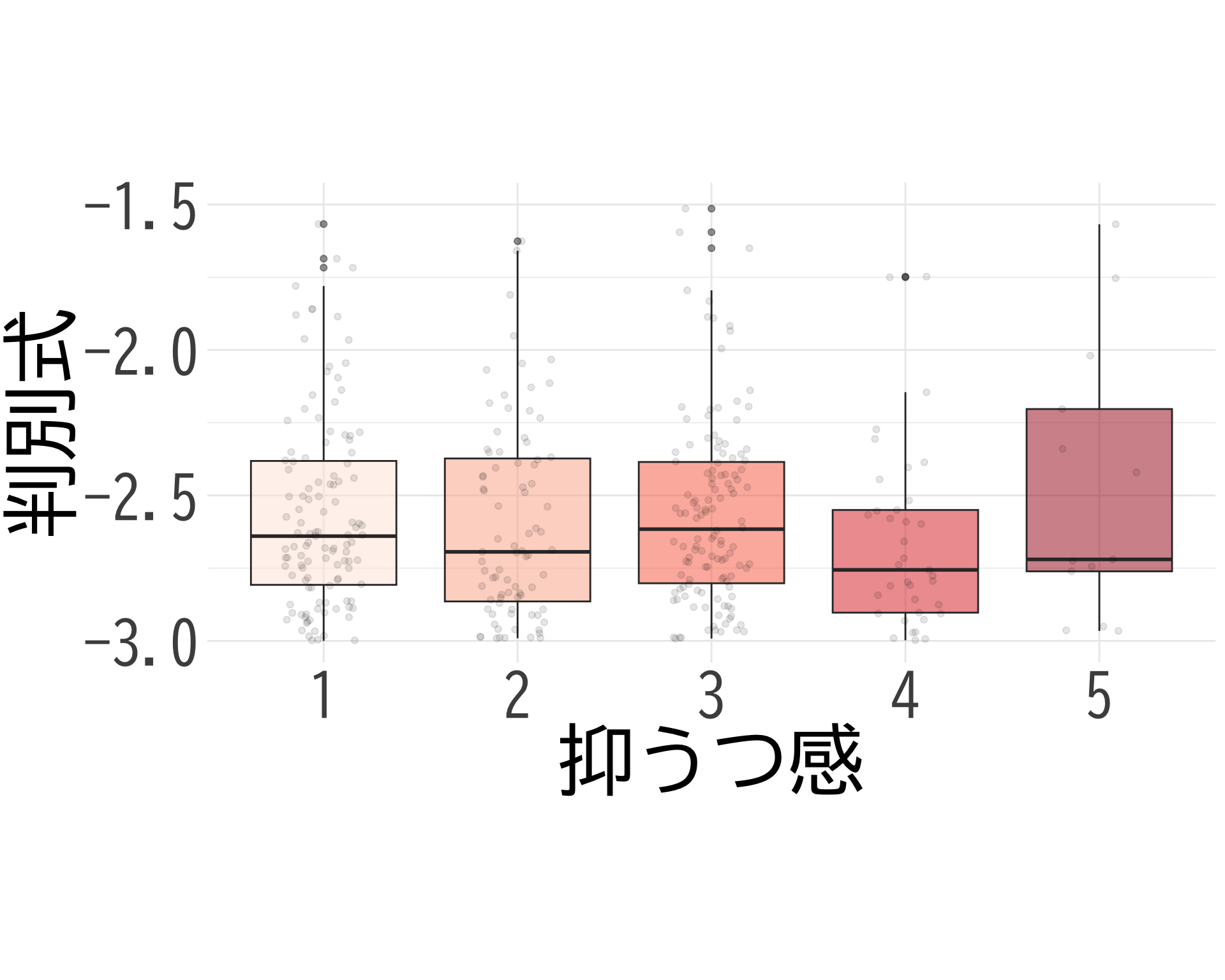
抑うつ感×判別式
# データの準備(BP_A_flag = 0 の行のみ選択) <- data.frame (= factor (df$ 抑うつ感[df$ BP_A_flag == 0 & ! is.na (df$ 抑うつ感)], levels = 1 : 5 ,labels = 1 : 5 ),= df$ 判別式[df$ BP_A_flag == 0 & ! is.na (df$ 抑うつ感)]# ggplotでプロット ggplot (judge_by_抑うつ感, aes (x = 抑うつ感, y = 判別式, fill = 抑うつ感)) + geom_boxplot (alpha = 0.5 ) + geom_jitter (width = 0.2 , alpha = 0.1 ) + theme_minimal () + labs (x = "抑うつ感" ,y = "判別式" ) + theme (text = element_text (family = "BIZUDGothic-Regular" , size = 16 ), # 基本フォントサイズを16に axis.text = element_text (size = 34 ),axis.title = element_text (size = 45 ),legend.position = "none" + scale_fill_brewer (palette = "Reds" ) + scale_y_continuous (limits = c (- 3 , - 1.5 )) + coord_fixed (ratio = 1.5 )
Warning: Removed 749 rows containing non-finite values (`stat_boxplot()`).
Warning: Removed 750 rows containing missing values (`geom_point()`).
# ggsave("抑うつ感×判別式.png", bg="white")
これでも \(p\) -値が出ない.
# データの抽出(BP_A_flag = 0 かつ item2 が 1 または 2 のデータ) <- df$ 判別式[df$ BP_A_flag == 0 & df$ 抑うつ感 == 1 ]<- df$ 判別式[df$ BP_A_flag == 0 & df$ 抑うつ感 == 5 ]# 等分散性の検定(Levene検定) var.test (bp_抑うつ感_1, bp_抑うつ感_2)
    F test to compare two variances

data:  bp_抑うつ感_1 and bp_抑うつ感_2
F = 0.029822, num df = 363, denom df = 27, p-value < 2.2e-16
alternative hypothesis: true ratio of variances is not equal to 1
95 percent confidence interval:
 0.01587170 0.04890551
sample estimates:
ratio of variances
        0.02982172
# t検定の実施 t.test (bp_抑うつ感_1, bp_抑うつ感_2, var.equal = FALSE , # 等分散を仮定しない(Welchのt検定) alternative = "two.sided" ) # 両側検定
    Welch Two Sample t-test

data:  bp_抑うつ感_1 and bp_抑うつ感_2
t = 0.7618, df = 27.124, p-value = 0.4528
alternative hypothesis: true difference in means is not equal to 0
95 percent confidence interval:
 -3.099174  6.760739
sample estimates:
mean of x mean of y
-3.906824 -5.737607
Flag の情報が重要かもしれない
そこで,BP備考が NA のデータを抽出し,完全ケース分析をしてみる.
<- df[is.na (df$ BP備考), ]
疲労感:お?
# データの準備(BP_A_flag = 0 の行のみ選択) <- data.frame (= factor (df_na_BP備考$ 疲労感[df_na_BP備考$ BP_A_flag == 0 & ! is.na (df_na_BP備考$ 疲労感)], levels = 1 : 5 ,labels = 1 : 5 ),BP = df_na_BP備考$ BP[df_na_BP備考$ BP_A_flag == 0 & ! is.na (df_na_BP備考$ 疲労感)]# ggplotでプロット ggplot (judge_by_疲労感, aes (x = 疲労感, y = BP, fill = 疲労感)) + geom_boxplot (alpha = 0.5 ) + geom_jitter (width = 0.2 , alpha = 0.1 ) + theme_minimal () + labs (title = "疲労感の回答別BPの分布" ,x = "疲労感" ,y = "BP" ) + theme (text = element_text (family = "BIZUDGothic-Regular" , size = 16 ), # 基本フォントサイズを16に axis.text = element_text (size = 14 ), # 軸の目盛りの文字サイズ axis.title = element_text (size = 18 ), # 軸タイトルの文字サイズ plot.title = element_text (size = 20 ), # プロットタイトルの文字サイズ legend.position = "none" + scale_fill_brewer (palette = "Reds" ) + scale_y_continuous (limits = c (0 , 2.5 )) # y軸の範囲を-2.5から2.5に設定
Warning: Removed 10 rows containing non-finite values (`stat_boxplot()`).
Warning: Removed 10 rows containing missing values (`geom_point()`).
# データの抽出(BP_A_flag = 0 かつ item2 が 1 または 2 のデータ) <- df_na_BP備考$ BP[df_na_BP備考$ BP_A_flag == 0 & df_na_BP備考$ 疲労感 == 1 ]<- df_na_BP備考$ BP[df_na_BP備考$ BP_A_flag == 0 & df_na_BP備考$ 疲労感 == 5 ]# 等分散性の検定(Levene検定) var.test (bp_疲労感_1, bp_疲労感_2)
    F test to compare two variances

data:  bp_疲労感_1 and bp_疲労感_2
F = 0.90489, num df = 116, denom df = 13, p-value = 0.7235
alternative hypothesis: true ratio of variances is not equal to 1
95 percent confidence interval:
 0.3400331 1.8256055
sample estimates:
ratio of variances
         0.9048891
# t検定の実施 t.test (bp_疲労感_1, bp_疲労感_2, var.equal = FALSE , # 等分散を仮定しない(Welchのt検定) alternative = "two.sided" ) # 両側検定
    Welch Two Sample t-test

data:  bp_疲労感_1 and bp_疲労感_2
t = -1.735, df = 15.947, p-value = 0.102
alternative hypothesis: true difference in means is not equal to 0
95 percent confidence interval:
 -0.5075630  0.0507498
sample estimates:
mean of x mean of y
0.8123077 1.0407143
疲労感×判別式
# データの準備(BP_A_flag = 0 の行のみ選択) <- data.frame (= factor (df_na_BP備考$ 疲労感[df_na_BP備考$ BP_A_flag == 0 & ! is.na (df_na_BP備考$ 疲労感)], levels = 1 : 5 ,labels = 1 : 5 ),= df_na_BP備考$ 判別式[df_na_BP備考$ BP_A_flag == 0 & ! is.na (df_na_BP備考$ 疲労感)]# ggplotでプロット ggplot (judge_by_疲労感, aes (x = 疲労感, y = 判別式, fill = 疲労感)) + geom_boxplot (alpha = 0.5 ) + geom_jitter (width = 0.2 , alpha = 0.1 ) + theme_minimal () + labs (title = "疲労感の回答別判別式の分布" ,x = "疲労感" ,y = "判別式" ) + theme (text = element_text (family = "BIZUDGothic-Regular" , size = 16 ), # 基本フォントサイズを16に axis.text = element_text (size = 14 ), # 軸の目盛りの文字サイズ axis.title = element_text (size = 18 ), # 軸タイトルの文字サイズ plot.title = element_text (size = 20 ), # プロットタイトルの文字サイズ legend.position = "none" + scale_fill_brewer (palette = "Reds" ) + scale_y_continuous (limits = c (- 2.5 , 0 )) # y軸の範囲を-2.5から2.5に設定
Warning: Removed 526 rows containing non-finite values (`stat_boxplot()`).
Warning: Removed 526 rows containing missing values (`geom_point()`).
これだと \(p\) -値が出なくなる.
# データの抽出(BP_A_flag = 0 かつ item2 が 1 または 2 のデータ) <- df_na_BP備考$ 判別式[df_na_BP備考$ BP_A_flag == 0 & df_na_BP備考$ 疲労感 == 1 ]<- df_na_BP備考$ 判別式[df_na_BP備考$ BP_A_flag == 0 & df_na_BP備考$ 疲労感 == 5 ]# 等分散性の検定(Levene検定) var.test (bp_疲労感_1, bp_疲労感_2)
    F test to compare two variances

data:  bp_疲労感_1 and bp_疲労感_2
F = 1.8943, num df = 116, denom df = 13, p-value = 0.1935
alternative hypothesis: true ratio of variances is not equal to 1
95 percent confidence interval:
 0.7118207 3.8216976
sample estimates:
ratio of variances
          1.894282
# t検定の実施 t.test (bp_疲労感_1, bp_疲労感_2, var.equal = FALSE , # 等分散を仮定しない(Welchのt検定) alternative = "two.sided" ) # 両側検定
    Welch Two Sample t-test

data:  bp_疲労感_1 and bp_疲労感_2
t = -1.9392, df = 19.449, p-value = 0.06712
alternative hypothesis: true difference in means is not equal to 0
95 percent confidence interval:
 -0.88779262  0.03317357
sample estimates:
mean of x mean of y
-3.404667 -2.977357
不安感:おお!?
# データの準備(BP_A_flag = 0 の行のみ選択) <- data.frame (= factor (df_na_BP備考$ 不安感[df_na_BP備考$ BP_A_flag == 0 & ! is.na (df_na_BP備考$ 不安感)], levels = 1 : 5 ,labels = 1 : 5 ),BP = df_na_BP備考$ BP[df_na_BP備考$ BP_A_flag == 0 & ! is.na (df_na_BP備考$ 不安感)]# ggplotでプロット ggplot (judge_by_不安感, aes (x = 不安感, y = BP, fill = 不安感)) + geom_boxplot (alpha = 0.5 ) + geom_jitter (width = 0.2 , alpha = 0.1 ) + theme_minimal () + labs (x = "不安感" ,y = "BP" ) + theme (text = element_text (family = "BIZUDGothic-Regular" , size = 16 ), # 基本フォントサイズを16に axis.text = element_text (size = 34 ),axis.title = element_text (size = 45 ),legend.position = "none" + scale_fill_brewer (palette = "Reds" ) + scale_y_continuous (limits = c (0.5 , 1.5 )) + coord_fixed (ratio = 2.1 )
Warning: Removed 109 rows containing non-finite values (`stat_boxplot()`).
Warning: Removed 112 rows containing missing values (`geom_point()`).
# ggsave("不安感_備考なし.png", bg="white")
# データの抽出(BP_A_flag = 0 かつ item2 が 1 または 2 のデータ) <- df_na_BP備考$ BP[df_na_BP備考$ BP_A_flag == 0 & df_na_BP備考$ 不安感 == 1 ]<- df_na_BP備考$ BP[df_na_BP備考$ BP_A_flag == 0 & df_na_BP備考$ 不安感 == 5 ]# 等分散性の検定(Levene検定) var.test (bp_不安感_1, bp_不安感_2)
    F test to compare two variances

data:  bp_不安感_1 and bp_不安感_2
F = 0.34031, num df = 194, denom df = 13, p-value = 0.001257
alternative hypothesis: true ratio of variances is not equal to 1
95 percent confidence interval:
 0.1291465 0.6706941
sample estimates:
ratio of variances
         0.3403088
# t検定の実施 t.test (bp_不安感_1, bp_不安感_2, var.equal = FALSE , # 等分散を仮定しない(Welchのt検定) alternative = "two.sided" ) # 両側検定
    Welch Two Sample t-test

data:  bp_不安感_1 and bp_不安感_2
t = -0.99191, df = 13.642, p-value = 0.3385
alternative hypothesis: true difference in means is not equal to 0
95 percent confidence interval:
 -0.4439628  0.1636477
sample estimates:
mean of x mean of y
0.8091282 0.9492857
Warning: パッケージ 'BayesFactor' はバージョン 4.3.1 の R の下で造られました
************
Welcome to BayesFactor 0.9.12-4.7. If you have questions, please contact Richard Morey (richarddmorey@gmail.com).

Type BFManual() to open the manual.
************
次のパッケージを付け加えます: 'BayesFactor'
 以下のオブジェクトは 'package:igraph' からマスクされています:

    compare
# NAを除外したデータの作成 <- na.omit (bp_不安感_1)<- na.omit (bp_不安感_2)# ベイズ因子の計算 library (BayesFactor)<- ttestBF (x = bp_不安感_1_clean, y = bp_不安感_2_clean,paired = FALSE ,rscale = "medium" )# 結果の表示 print (bf)
Bayes factor analysis
--------------
[1] Alt., r=0.707 : 0.764421 ±0.01%

Against denominator:
  Null, mu1-mu2 = 0
---
Bayes factor type: BFindepSample, JZS
# サンプルサイズの確認 cat (" \n サンプルサイズ: \n " )cat ("グループ1:" , length (bp_不安感_1_clean), " \n " )cat ("グループ2:" , length (bp_不安感_2_clean), " \n " )
全く備考情報を考慮しないと?
<- df$ BP[df$ 不安感 == 1 ]<- df$ BP[df$ 不安感 == 5 ]# NAを除外したデータの作成 <- na.omit (bp_不安感_1)<- na.omit (bp_不安感_2)# ベイズ因子の計算 library (BayesFactor)<- ttestBF (x = bp_不安感_1_clean, y = bp_不安感_2_clean,paired = FALSE ,rscale = "medium" )# 結果の表示 print (bf)
Bayes factor analysis
--------------
[1] Alt., r=0.707 : 0.2298194 ±0.02%

Against denominator:
  Null, mu1-mu2 = 0
---
Bayes factor type: BFindepSample, JZS
# サンプルサイズの確認 cat (" \n サンプルサイズ: \n " )cat ("グループ1:" , length (bp_不安感_1_clean), " \n " )cat ("グループ2:" , length (bp_不安感_2_clean), " \n " )
不安感×判別式
やはり判別式も有意に低いが,少し分散が大きくなる.
# データの準備(BP_A_flag = 0 の行のみ選択) <- data.frame (= factor (df_na_BP備考$ 不安感[df_na_BP備考$ BP_A_flag == 0 & ! is.na (df_na_BP備考$ 不安感)], levels = 1 : 5 ,labels = 1 : 5 ),= df_na_BP備考$ 判別式[df_na_BP備考$ BP_A_flag == 0 & ! is.na (df_na_BP備考$ 不安感)]# ggplotでプロット ggplot (judge_by_不安感, aes (x = 不安感, y = 判別式, fill = 不安感)) + geom_boxplot (alpha = 0.5 ) + geom_jitter (width = 0.2 , alpha = 0.1 ) + theme_minimal () + labs (title = "不安感の回答別判別式の分布" ,x = "不安感" ,y = "判別式" ) + theme (text = element_text (family = "BIZUDGothic-Regular" , size = 16 ), # 基本フォントサイズを16に axis.text = element_text (size = 14 ), # 軸の目盛りの文字サイズ axis.title = element_text (size = 18 ), # 軸タイトルの文字サイズ plot.title = element_text (size = 20 ), # プロットタイトルの文字サイズ legend.position = "none" + scale_fill_brewer (palette = "Reds" ) + scale_y_continuous (limits = c (- 3 , 0 )) # y軸の範囲を-2.5から2.5に設定
Warning: Removed 402 rows containing non-finite values (`stat_boxplot()`).
Warning: Removed 403 rows containing missing values (`geom_point()`).
# データの抽出(BP_A_flag = 0 かつ item2 が 1 または 2 のデータ) <- df_na_BP備考$ 判別式[df_na_BP備考$ BP_A_flag == 0 & df_na_BP備考$ 不安感 == 1 ]<- df_na_BP備考$ 判別式[df_na_BP備考$ BP_A_flag == 0 & df_na_BP備考$ 不安感 == 5 ]# 等分散性の検定(Levene検定) var.test (bp_不安感_1, bp_不安感_2)
    F test to compare two variances

data:  bp_不安感_1 and bp_不安感_2
F = 2.2447, num df = 194, denom df = 13, p-value = 0.09829
alternative hypothesis: true ratio of variances is not equal to 1
95 percent confidence interval:
 0.8518462 4.4238763
sample estimates:
ratio of variances
          2.244666
# t検定の実施 t.test (bp_不安感_1, bp_不安感_2, var.equal = FALSE , # 等分散を仮定しない(Welchのt検定) alternative = "two.sided" ) # 両側検定
    Welch Two Sample t-test

data:  bp_不安感_1 and bp_不安感_2
t = -2.0503, df = 17.497, p-value = 0.05562
alternative hypothesis: true difference in means is not equal to 0
95 percent confidence interval:
 -0.90811613  0.01200331
sample estimates:
mean of x mean of y
-3.579056 -3.131000
BP 値の方が分散が違うが,判別式の方が \(p\) -値が小さい
判別式はすごい出るが,\(p<0.05\) まではいかない.一方で,測定できない以上が出たという情報まで入れると有意性が出てくる.
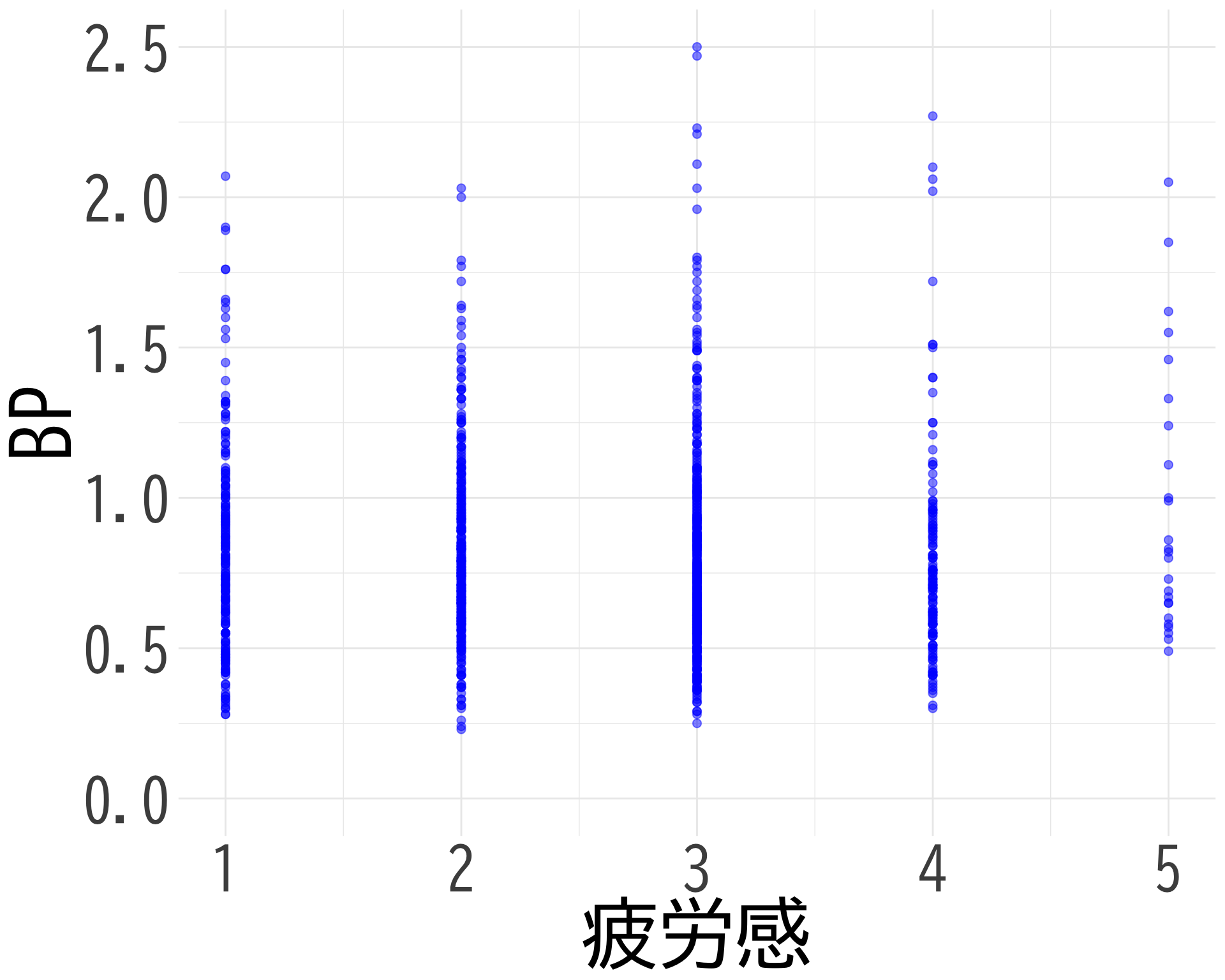
疲労感と BP の散布図
# データの準備(NAを除外) <- data.frame (= df$ 疲労感[df$ BP_A_flag == 0 & ! is.na (df$ 疲労感) & ! is.na (df$ BP)],BP = df$ BP[df$ BP_A_flag == 0 & ! is.na (df$ 疲労感) & ! is.na (df$ BP)]# 散布図の作成 ggplot (scatter_data, aes (x = 疲労感, y = BP)) + geom_point (alpha = 0.5 , color = "blue" , size = 2 ) + theme_minimal () + labs (x = "疲労感" ,y = "BP" ) + theme (text = element_text (family = "BIZUDGothic-Regular" , size = 16 ),axis.text = element_text (size = 34 ),axis.title = element_text (size = 45 ),+ scale_x_continuous (breaks = 1 : 5 ) + scale_y_continuous (limits = c (0.0 , 2.5 ))
Warning: Removed 5 rows containing missing values (`geom_point()`).
ggsave ("疲労感とBPの散布図.png" , bg= "white" )
Warning: Removed 5 rows containing missing values (`geom_point()`).
不安感と BP の散布図
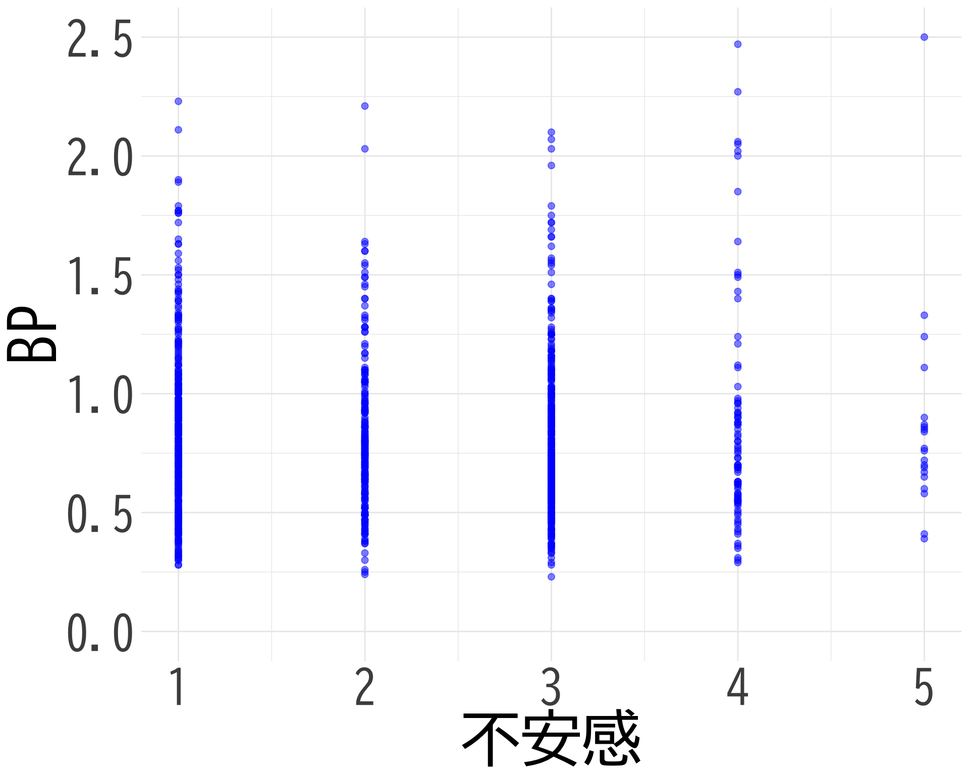
# データの準備(NAを除外) <- data.frame (= df$ 不安感[df$ BP_A_flag == 0 & ! is.na (df$ 不安感) & ! is.na (df$ BP)],BP = df$ BP[df$ BP_A_flag == 0 & ! is.na (df$ 不安感) & ! is.na (df$ BP)]# 散布図の作成 ggplot (scatter_data, aes (x = 不安感, y = BP)) + geom_point (alpha = 0.5 , color = "blue" , size = 2 ) + theme_minimal () + labs (x = "不安感" ,y = "BP" ) + theme (text = element_text (family = "BIZUDGothic-Regular" , size = 16 ),axis.text = element_text (size = 34 ),axis.title = element_text (size = 45 ),+ scale_x_continuous (breaks = 1 : 5 ) + scale_y_continuous (limits = c (0.0 , 2.5 ))
Warning: Removed 5 rows containing missing values (`geom_point()`).
ggsave ("不安感とBPの散布図.png" , bg= "white" )
Warning: Removed 5 rows containing missing values (`geom_point()`).
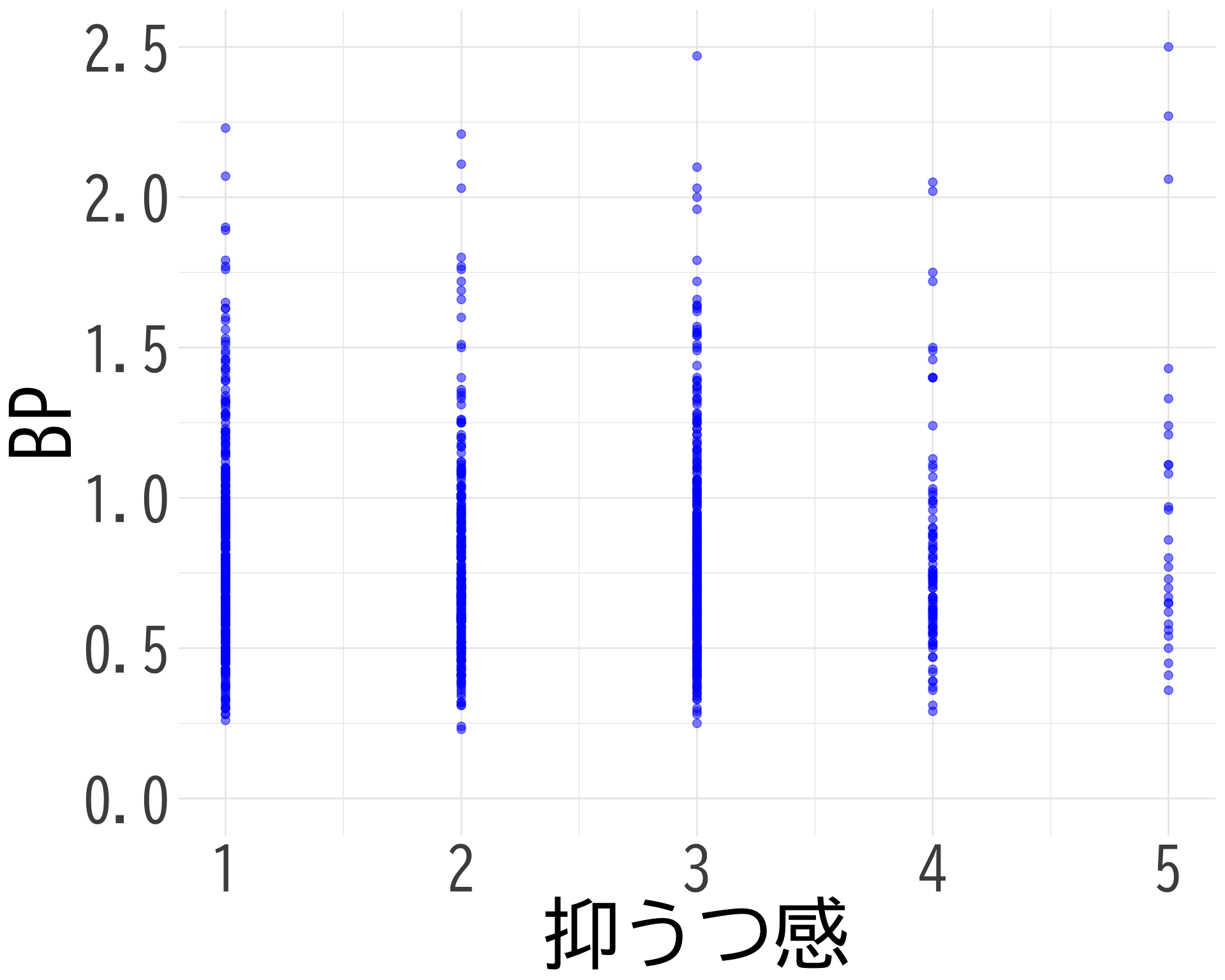
抑うつ感と BP の散布図
# データの準備(NAを除外) <- data.frame (= df$ 抑うつ感[df$ BP_A_flag == 0 & ! is.na (df$ 抑うつ感) & ! is.na (df$ BP)],BP = df$ BP[df$ BP_A_flag == 0 & ! is.na (df$ 抑うつ感) & ! is.na (df$ BP)]# 散布図の作成 ggplot (scatter_data, aes (x = 抑うつ感, y = BP)) + geom_point (alpha = 0.5 , color = "blue" , size = 2 ) + theme_minimal () + labs (x = "抑うつ感" ,y = "BP" ) + theme (text = element_text (family = "BIZUDGothic-Regular" , size = 16 ),axis.text = element_text (size = 34 ),axis.title = element_text (size = 45 ),+ scale_x_continuous (breaks = 1 : 5 ) + scale_y_continuous (limits = c (0.0 , 2.5 ))
Warning: Removed 5 rows containing missing values (`geom_point()`).
ggsave ("抑うつ感とBPの散布図.png" , bg= "white" )
Warning: Removed 5 rows containing missing values (`geom_point()`).
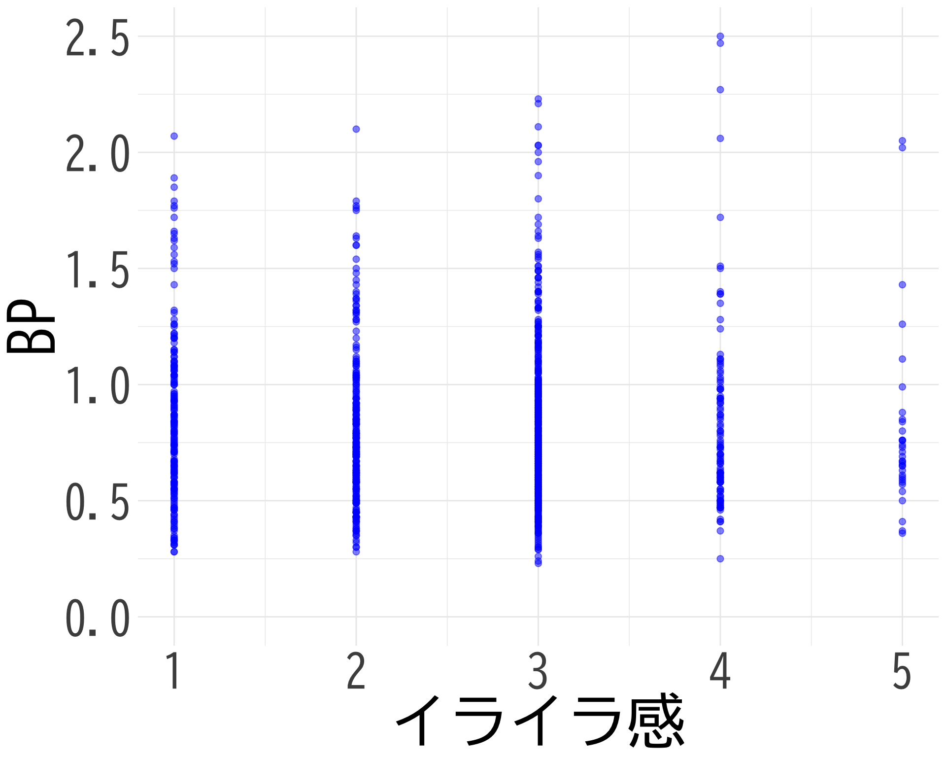
イライラ感と BP の散布図
# データの準備(NAを除外) <- data.frame (= df$ イライラ感[df$ BP_A_flag == 0 & ! is.na (df$ イライラ感) & ! is.na (df$ BP)],BP = df$ BP[df$ BP_A_flag == 0 & ! is.na (df$ イライラ感) & ! is.na (df$ BP)]# 散布図の作成 ggplot (scatter_data, aes (x = イライラ感, y = BP)) + geom_point (alpha = 0.5 , color = "blue" , size = 2 ) + theme_minimal () + labs (x = "イライラ感" ,y = "BP" ) + theme (text = element_text (family = "BIZUDGothic-Regular" , size = 16 ),axis.text = element_text (size = 34 ),axis.title = element_text (size = 45 ),+ scale_x_continuous (breaks = 1 : 5 ) + scale_y_continuous (limits = c (0.0 , 2.5 ))
Warning: Removed 5 rows containing missing values (`geom_point()`).
ggsave ("イライラ感とBPの散布図.png" , bg= "white" )
Warning: Removed 5 rows containing missing values (`geom_point()`).
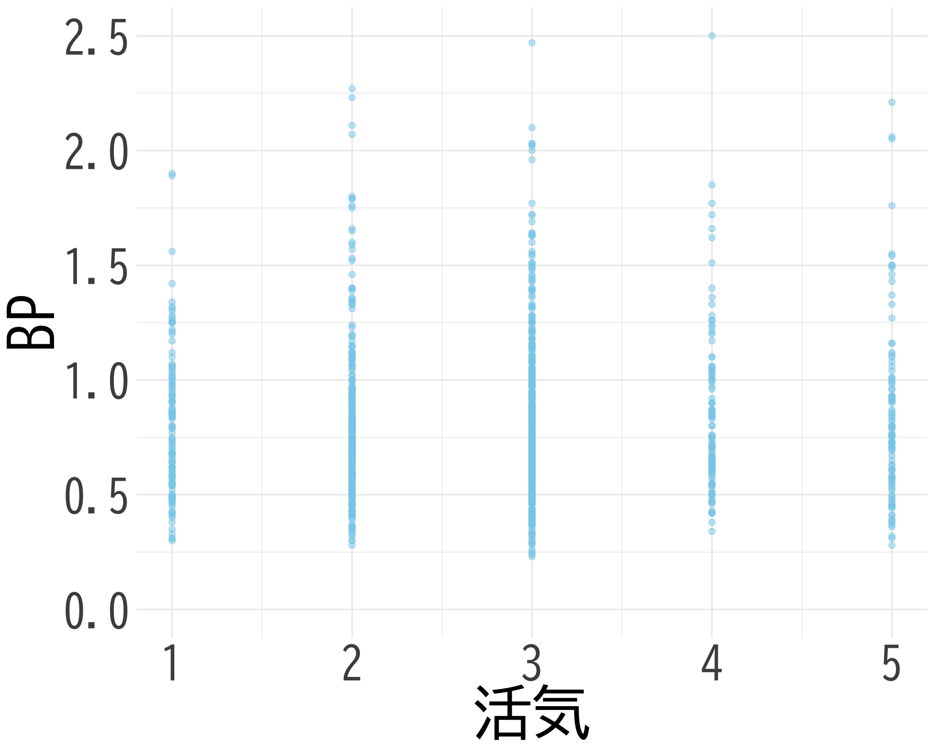
活気と BP の散布図
# データの準備(NAを除外) <- data.frame (= df$ 活気[df$ BP_A_flag == 0 & ! is.na (df$ 活気) & ! is.na (df$ BP)],BP = df$ BP[df$ BP_A_flag == 0 & ! is.na (df$ 活気) & ! is.na (df$ BP)]# 散布図の作成 ggplot (scatter_data, aes (x = 活気, y = BP)) + geom_point (alpha = 0.5 , color = "skyblue" , size = 2 ) + theme_minimal () + labs (x = "活気" ,y = "BP" ) + theme (text = element_text (family = "BIZUDGothic-Regular" , size = 16 ),axis.text = element_text (size = 34 ),axis.title = element_text (size = 45 ),+ scale_x_continuous (breaks = 1 : 5 ) + scale_y_continuous (limits = c (0.0 , 2.5 ))
Warning: Removed 5 rows containing missing values (`geom_point()`).
# ggsave("活気とBPの散布図.png", bg="white")
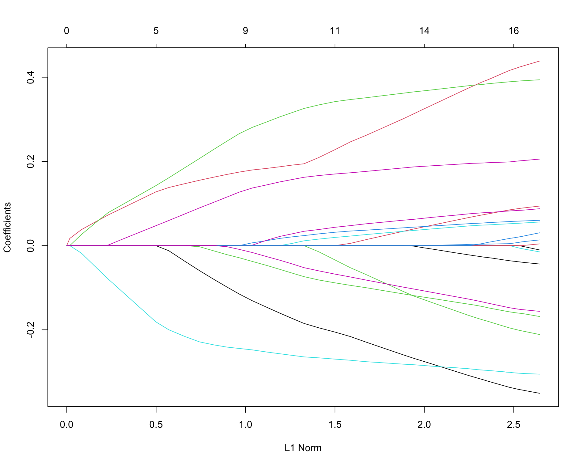
LASSO をやってみる
library (glmnet)<- df$ 判別式<- df[, paste0 ("item" , 1 : 18 )]# 前処理の確認 print (head (df$ 判別式)) # 元の判別式の値を確認
[1] -2.880 -3.343 -2.727 -2.974 -7.338 -2.776
# 完全なケースのみを抽出 <- complete.cases (x) & ! is.na (y)<- x[complete_cases, ]<- y[complete_cases]# データの次元を確認 print (dim (x_complete))print (length (y_complete))# y_completeの要約統計量 print (summary (y_complete))
   Min. 1st Qu.  Median    Mean 3rd Qu.    Max.
-70.246  -4.207  -3.295  -3.976  -2.796   3.120
# GLMNETを実行 <- glmnet (as.matrix (x_complete), y_complete)plot (fit)
item2:「元気がいっぱいだ」
item9:「だるい」
item17 (-):「仕事が手につかない」
item6:「イライラしている」
職業性ストレスチェックでは何も説明できていないことが如実に現れている.
Call:  glmnet(x = as.matrix(x_complete), y = y_complete)

   Df %Dev   Lambda
1   0 0.00 0.163900
2   1 0.04 0.149300
3   3 0.17 0.136000
4   3 0.30 0.124000
5   4 0.41 0.112900
6   4 0.51 0.102900
7   4 0.60 0.093770
8   4 0.67 0.085440
9   4 0.74 0.077850
10  5 0.81 0.070940
11  5 0.89 0.064630
12  6 0.96 0.058890
13  6 1.02 0.053660
14  7 1.08 0.048890
15  7 1.12 0.044550
16  9 1.16 0.040590
17  9 1.21 0.036990
18  9 1.24 0.033700
19 10 1.27 0.030710
20 10 1.30 0.027980
21 11 1.33 0.025490
22 11 1.36 0.023230
23 12 1.39 0.021160
24 12 1.41 0.019280
25 12 1.43 0.017570
26 12 1.45 0.016010
27 12 1.46 0.014590
28 13 1.47 0.013290
29 14 1.48 0.012110
30 14 1.49 0.011040
31 14 1.50 0.010050
32 14 1.51 0.009162
33 14 1.51 0.008348
34 14 1.51 0.007606
35 14 1.52 0.006930
36 15 1.52 0.006315
37 15 1.52 0.005754
38 15 1.53 0.005243
39 15 1.53 0.004777
40 15 1.53 0.004353
41 15 1.53 0.003966
42 15 1.53 0.003614
43 15 1.53 0.003293
44 15 1.53 0.003000
45 15 1.53 0.002734
46 16 1.53 0.002491
47 16 1.53 0.002269
48 16 1.53 0.002068
49 16 1.53 0.001884
50 16 1.53 0.001717
51 17 1.54 0.001564
52 18 1.54 0.001425
53 18 1.54 0.001299
54 18 1.54 0.001183
55 18 1.54 0.001078
56 18 1.54 0.000982
57 18 1.54 0.000895
58 18 1.54 0.000816
59 18 1.54 0.000743
60 18 1.54 0.000677
61 18 1.54 0.000617
62 18 1.54 0.000562
63 18 1.54 0.000512
64 18 1.54 0.000467
65 18 1.54 0.000425
66 18 1.54 0.000388
67 18 1.54 0.000353
68 18 1.54 0.000322
19 x 1 sparse Matrix of class "dgCMatrix"
                     s1
(Intercept) -4.26588492
item1        .
item2        0.09301905
item3        .
item4        .
item5        .
item6        0.01848971
item7        .
item8        .
item9        0.10196089
item10       .
item11       .
item12       .
item13       .
item14       .
item15       .
item16       .
item17      -0.11706724
item18       .
Graphical Lasso をやってみる
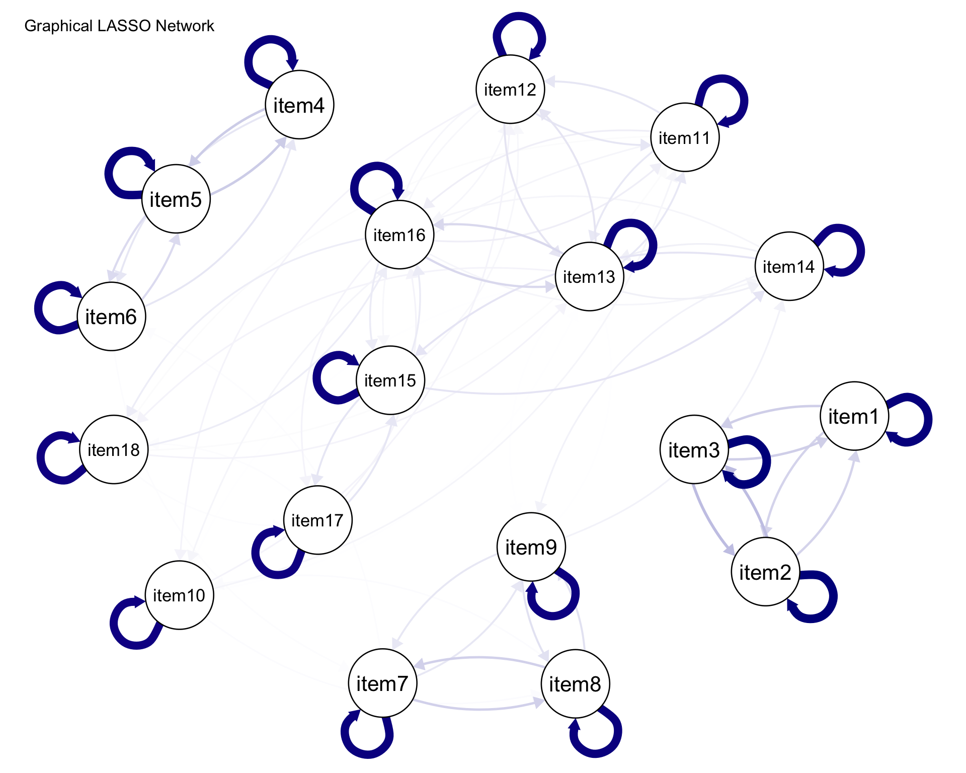
library (glasso)# 相関行列の計算 # 完全なケースのみを使用 <- cor (x_complete)# Graphical LASSOの実行 # rhoは正則化パラメータ。小さいほど密なネットワーク、大きいほど疎なネットワークになります <- glasso (x_cor, rho = 0.5 )# 結果の確認 # 精度行列(逆共分散行列) <- glasso_result$ wi# 推定された共分散行列 <- glasso_result$ w# ネットワークの可視化 library (qgraph)library (igraph)# qgraphを使用してネットワークを可視化 qgraph (precision_matrix, layout = "spring" ,labels = paste0 ("item" , 1 : 18 ),edge.color = "darkblue" ,title = "Graphical LASSO Network" )
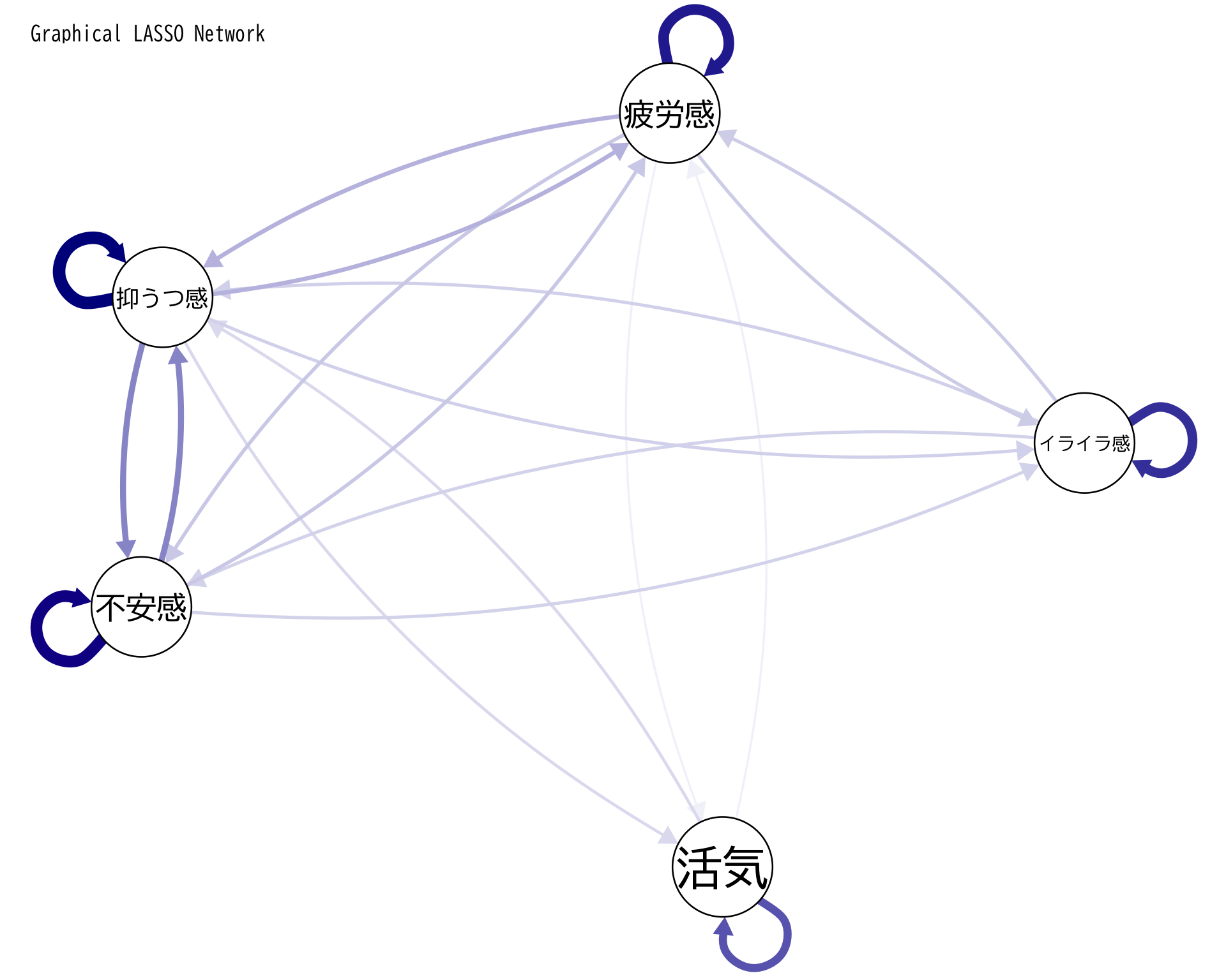
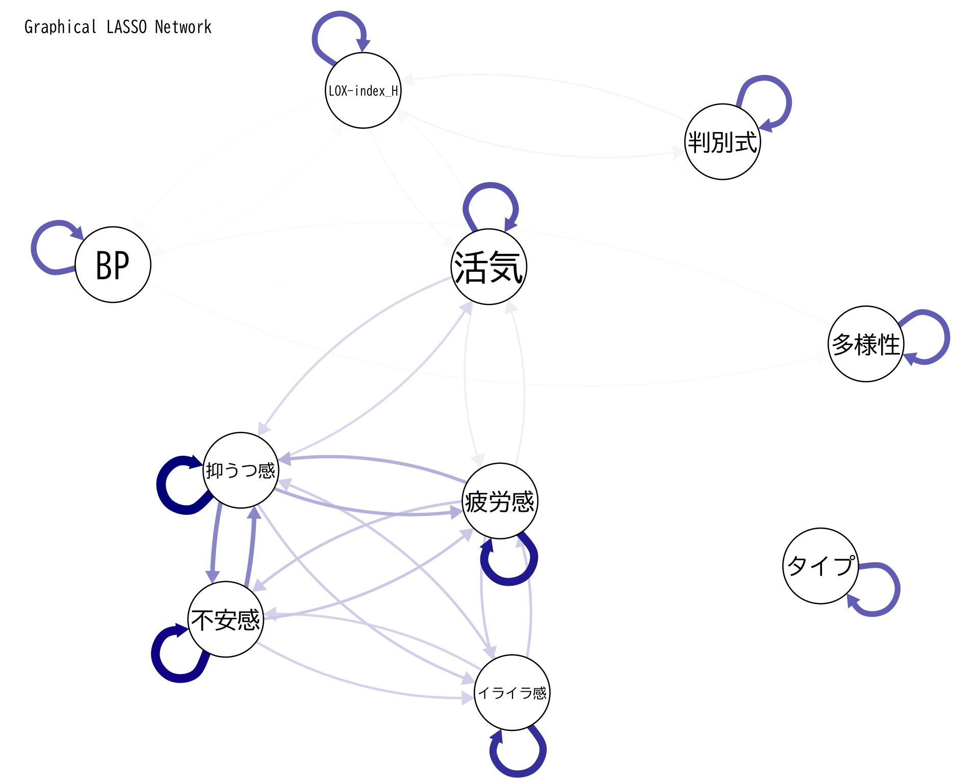
<- df[, c ("活気" , "イライラ感" , "疲労感" , "不安感" , "抑うつ感" )]<- x[complete.cases (x), ]<- cor (x_complete)<- glasso (x_cor, rho = 0.05 )<- glasso_result$ wipar (family = "BIZUDGothic-Regular" )# qgraphでの表示(fontFamilyは削除) qgraph (precision_matrix, layout = "spring" ,labels = colnames (x),edge.color = "darkblue" ,title = "Graphical LASSO Network" ,label.font = 2 , # フォントの太さ label.scale = TRUE , # ラベルのサイズを自動調整 label.cex = 1.2 , # ラベルの文字サイズ label.norm = "0000" ) # 日本語文字の位置調整
抑うつ感と不安感は強く連動しているようだ.
プリメディカの3つのサービス間に,簡単な相関はみられない.
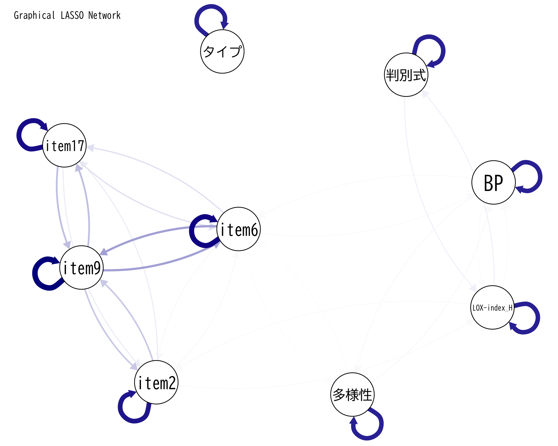
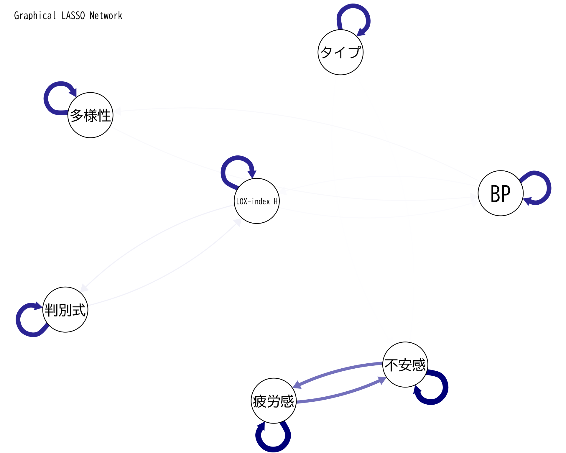
<- df[, c ("判別式" , "BP" , "LOX-index_H" , "タイプ" , "多様性" , paste0 ("item" , c (2 ,6 ,9 ,17 )))]$ タイプ <- as.numeric (factor (df$ タイプ, levels = c ("A" , "B" , "C" , "D" , "E" )))<- x[complete.cases (x), ]<- cor (x_complete)<- glasso (x_cor, rho = 0.05 )<- glasso_result$ wipar (family = "BIZUDGothic-Regular" )# qgraphでの表示(fontFamilyは削除) qgraph (precision_matrix, layout = "spring" ,labels = colnames (x),edge.color = "darkblue" ,title = "Graphical LASSO Network" ,label.font = 2 , # フォントの太さ label.scale = TRUE , # ラベルのサイズを自動調整 label.cex = 1.2 , # ラベルの文字サイズ label.norm = "0000" ) # 日本語文字の位置調整
<- df[, c ("判別式" , "BP" , "LOX-index_H" , "タイプ" , "多様性" , "活気" , "イライラ感" , "疲労感" , "不安感" , "抑うつ感" )]$ タイプ <- as.numeric (factor (df$ タイプ, levels = c ("A" , "B" , "C" , "D" , "E" )))<- x[complete.cases (x), ]<- cor (x_complete)<- glasso (x_cor, rho = 0.05 )<- glasso_result$ wipar (family = "BIZUDGothic-Regular" )# qgraphでの表示(fontFamilyは削除) qgraph (precision_matrix, layout = "spring" ,labels = colnames (x),edge.color = "darkblue" ,title = "Graphical LASSO Network" ,label.font = 2 , # フォントの太さ label.scale = TRUE , # ラベルのサイズを自動調整 label.cex = 1.2 , # ラベルの文字サイズ label.norm = "0000" ) # 日本語文字の位置調整
<- df[, c ("判別式" , "BP" , "LOX-index_H" , "タイプ" , "多様性" ,"疲労感" , "不安感" )]$ タイプ <- as.numeric (factor (df$ タイプ, levels = c ("A" , "B" , "C" , "D" , "E" )))<- x[complete.cases (x), ]<- cor (x_complete)<- glasso (x_cor, rho = 0.05 )<- glasso_result$ wipar (family = "BIZUDGothic-Regular" )# qgraphでの表示(fontFamilyは削除) qgraph (precision_matrix, layout = "spring" ,labels = colnames (x),edge.color = "darkblue" ,title = "Graphical LASSO Network" ,label.font = 2 , # フォントの太さ label.scale = TRUE , # ラベルのサイズを自動調整 label.cex = 1.2 , # ラベルの文字サイズ label.norm = "0000" ) # 日本語文字の位置調整
判別式と LOX の間の関係
全く線型関係ではないようであるし,背後に別の因子が関係しているようだ.
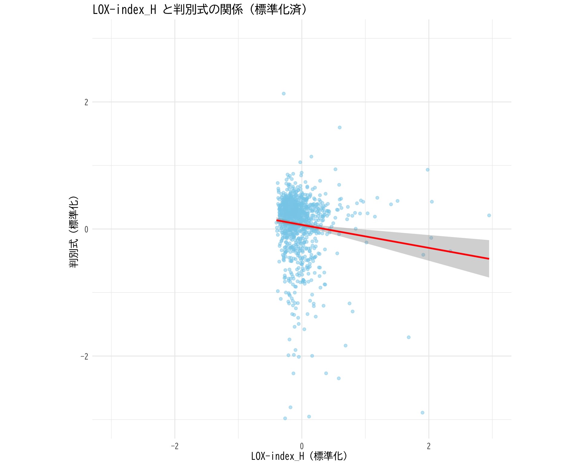
# BP_A_flag = 0 のデータを抽出 <- df[df$ BP_A_flag == 0 , ]# 標準化関数(NaNを考慮) <- function (x) {- mean (x, na.rm = TRUE )) / sd (x, na.rm = TRUE )# データフレームの作成(標準化したデータ) <- data.frame (LOX_index_H_std = standardize (df_filtered$ ` LOX-index_H ` ),_std = standardize (df_filtered$ 判別式)# 散布図 ggplot (plot_data, aes (x = LOX_index_H_std, y = 判別式_std)) + geom_point (alpha = 0.5 , color = "skyblue" ) + geom_smooth (method = "lm" , color = "red" , se = TRUE ) + theme_minimal () + labs (title = "LOX-index_H と判別式の関係(標準化済)" ,x = "LOX-index_H(標準化)" ,y = "判別式(標準化)" ) + theme (text = element_text (family = "BIZUDGothic-Regular" , size = 12 )+ # 両軸のスケールを同じに coord_fixed (ratio = 1 ) + # 軸の範囲を-3から3に設定(標準偏差の±3倍程度) scale_x_continuous (limits = c (- 3 , 3 )) + scale_y_continuous (limits = c (- 3 , 3 ))
`geom_smooth()` using formula = 'y ~ x'
Warning: Removed 50 rows containing non-finite values (`stat_smooth()`).
Warning: Removed 50 rows containing missing values (`geom_point()`).
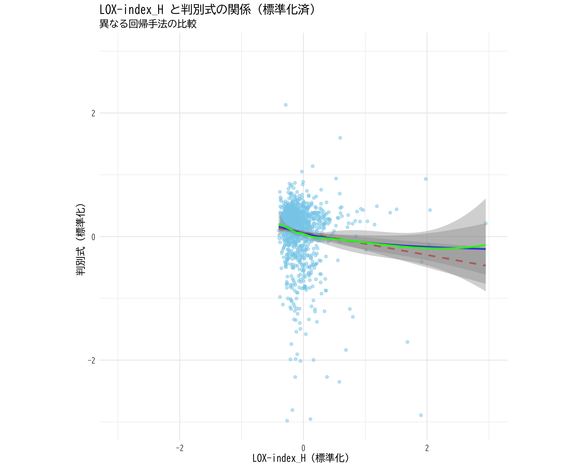
ggplot (plot_data, aes (x = LOX_index_H_std, y = 判別式_std)) + geom_point (alpha = 0.5 , color = "skyblue" ) + # 線形回帰 geom_smooth (method = "lm" , color = "red" , se = TRUE , linetype = "dashed" ) + # GAM(一般化加法モデル)による非線形回帰 geom_smooth (method = "gam" , color = "blue" , se = TRUE ) + # LOESS(局所回帰)による非線形回帰 geom_smooth (method = "loess" , color = "green" , se = TRUE ) + theme_minimal () + labs (title = "LOX-index_H と判別式の関係(標準化済)" ,subtitle = "異なる回帰手法の比較" ,x = "LOX-index_H(標準化)" ,y = "判別式(標準化)" ) + theme (text = element_text (family = "BIZUDGothic-Regular" , size = 12 )+ coord_fixed (ratio = 1 ) + scale_x_continuous (limits = c (- 3 , 3 )) + scale_y_continuous (limits = c (- 3 , 3 ))
`geom_smooth()` using formula = 'y ~ x'
Warning: Removed 50 rows containing non-finite values (`stat_smooth()`).
`geom_smooth()` using formula = 'y ~ s(x, bs = "cs")'
Warning: Removed 50 rows containing non-finite values (`stat_smooth()`).
`geom_smooth()` using formula = 'y ~ x'
Warning: Removed 50 rows containing non-finite values (`stat_smooth()`).
Warning: Removed 50 rows containing missing values (`geom_point()`).
trancation が見える
真のスケールはすごく小さくて,他は外れ値というべき?
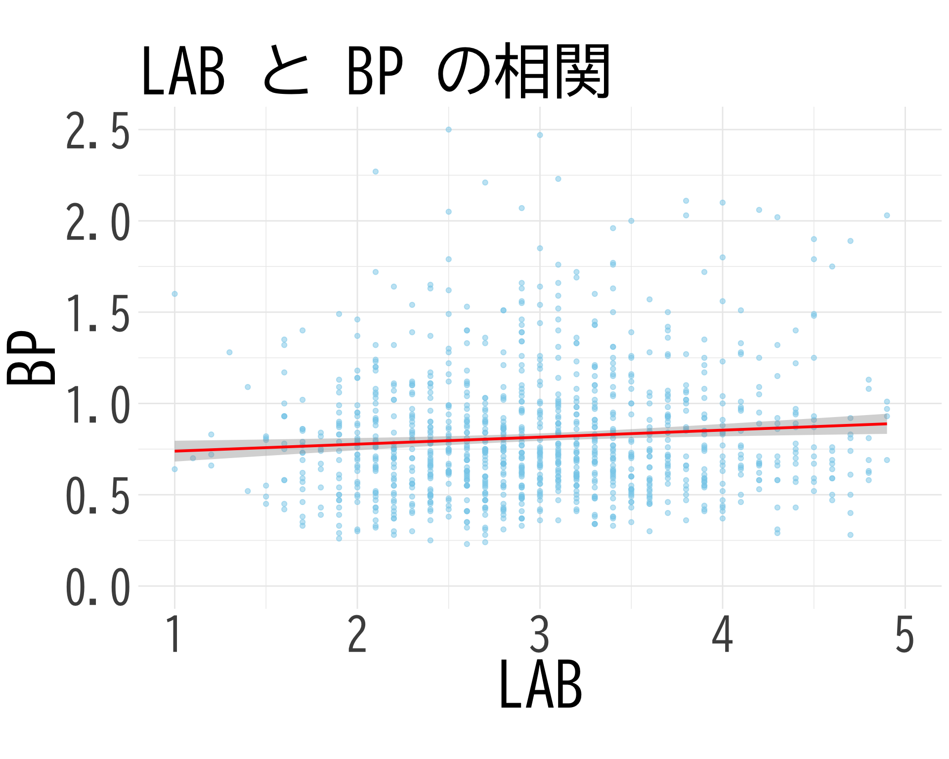
BP と LAB との関係
<- df[df$ BP_A_flag == 0 , c ("BP" , "LAB_H" )]colnames (mini_df) <- c ("BP" , "LAB" )summary (mini_df$ LAB)
   Min. 1st Qu.  Median    Mean 3rd Qu.    Max.    NA's
  0.900   2.400   3.000   3.022   3.500   6.400      29
ggplot (mini_df, aes (x = LAB, y = BP)) + geom_point (alpha = 0.5 , color = "skyblue" ) + geom_smooth (method = "lm" , color = "red" , se = TRUE ) + theme_minimal () + labs (title = "LAB と BP の相関" ,x = "LAB" ,y = "BP" ) + theme (text = element_text (family = "BIZUDGothic-Regular" , size = 12 ),axis.text = element_text (size = 34 ),axis.title = element_text (size = 45 ),plot.title = element_text (size = 45 )+ # 両軸のスケールを同じに coord_fixed (ratio = 1 ) + # 軸の範囲を-3から3に設定(標準偏差の±3倍程度) scale_x_continuous (limits = c (1 , 5 )) + scale_y_continuous (limits = c (0 , 2.5 ))
`geom_smooth()` using formula = 'y ~ x'
Warning: Removed 56 rows containing non-finite values (`stat_smooth()`).
Warning: Removed 56 rows containing missing values (`geom_point()`).
# ggsave("LABとBPの相関.png", bg="white")