弘前データ4:フローラスキャンデータの探索

著者

司馬博文

日付

5/24/2025

はじめに

hirosaki2.qmd では BP と LAB の関係のモデリング, hirosaki3.qmd では \(\Sigma\)-FLC と LOX-1 の関係をモデリングした. ここではフローラスキャンデータの探索を行う.

library(readxl)
library(knitr)
df <- readRDS("df.rds")
df <- df[is.na(df$`BP備考`), ]
kable(head(df))
id age sex Weight BP FLCΣ BP備考 判別式 LOX LAB LOX_Index type diversity BMI 年代 活気 イライラ感 疲労感 不安感 抑うつ感
3 4 46 1 76.3 1.10 1.95 NA -2.974 136 3.8 517 B 2 26.0 40代 2 3 2 3 2
5 6 30 1 59.5 0.76 0.64 NA -2.776 46 2.2 101 B 2 19.5 30代 3 5 4 5 4
6 7 51 1 76.6 1.69 2.58 NA -2.377 78 3.2 250 B 2 25.5 50代 3 3 3 3 2
7 8 47 2 43.2 0.56 0.55 NA -3.048 40 2.7 108 B 2 16.7 40代 2 1 2 2 1
9 10 39 1 61.9 0.52 0.64 NA -3.165 54 2.4 130 B 2 21.3 30代 3 3 3 3 3
10 11 55 1 61.0 0.89 2.64 NA -3.708 60 3.1 186 E 1 22.9 50代 3 2 2 1 1
df_IRT_long <- readRDS("df_IRT_long.rds")
df_IRT_long <- df_IRT_long[df_IRT_long$FLCΣ > 0, ]
kable(head(df_IRT_long))
id BP FLCΣ type diversity item response res
1 2 0.47 0.81 B 2 活気 3 0
2 2 0.47 0.81 B 2 イライラ感 3 0
3 2 0.47 0.81 B 2 疲労感 4 1
4 2 0.47 0.81 B 2 不安感 3 0
5 2 0.47 0.81 B 2 抑うつ感 3 0
11 4 1.10 1.95 B 2 活気 2 0

1 BP との関係

D は合計 \(6\) 人しかいない.

df <- subset(df, type != "D" & !is.na(diversity))
df$type <- droplevels(df$type)

1.1 視覚化

library(ggplot2)

ggplot(df, aes(x = type, fill = diversity)) +
    geom_bar(position = "fill") +
    geom_text(data = df, aes(label = ..count..), stat = "count", position = position_fill(vjust = 0.5)) +
  theme_minimal() +
  labs(title = "タイプ別の多様性の分布",
       x = "タイプ",
       y = "割合") +
  theme(text = element_text(family = "HiraKakuPro-W3"),
        plot.title = element_text(hjust = 0.5)) +
  scale_fill_manual(values = c(
    "1" = "#9999FF",    # 薄い青
    "2" = "#99FF99",  # 薄い緑
    "3" = "#FF9999"     # 薄い赤
  ))
Warning: The dot-dot notation (`..count..`) was deprecated in ggplot2 3.4.0.
ℹ Please use `after_stat(count)` instead.
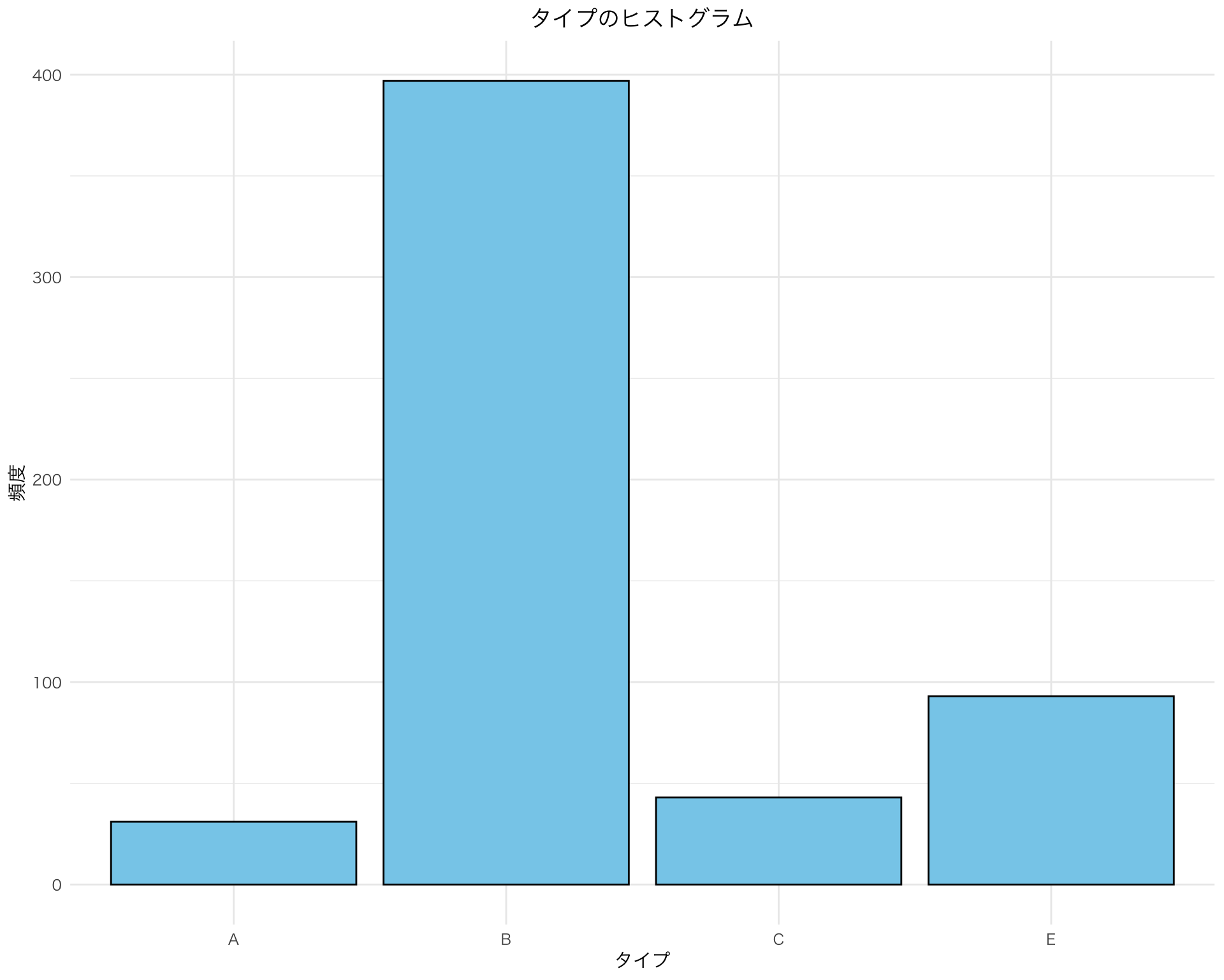
library(ggplot2)

ggplot(df, aes(x = type)) +
  geom_histogram(stat = "count", fill = "skyblue", color = "black") +
  theme_minimal() +
  labs(title = "タイプのヒストグラム",
       x = "タイプ",
       y = "頻度") +
  theme(text = element_text(family = "HiraKakuPro-W3"),
        plot.title = element_text(hjust = 0.5))
Warning in geom_histogram(stat = "count", fill = "skyblue", color = "black"):
Ignoring unknown parameters: `binwidth`, `bins`, and `pad`

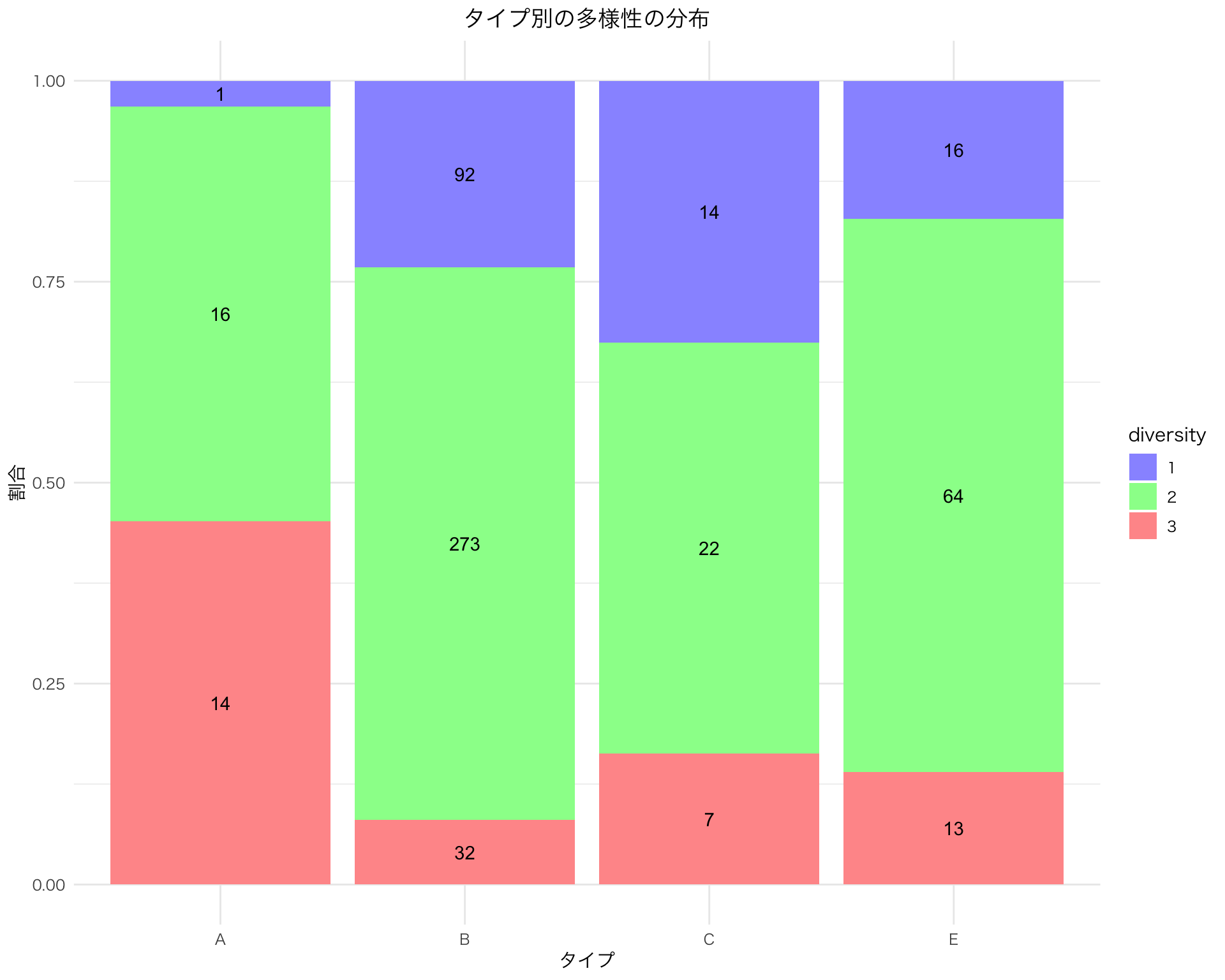
  • 明らかに type A は diversity 1 が少ない.
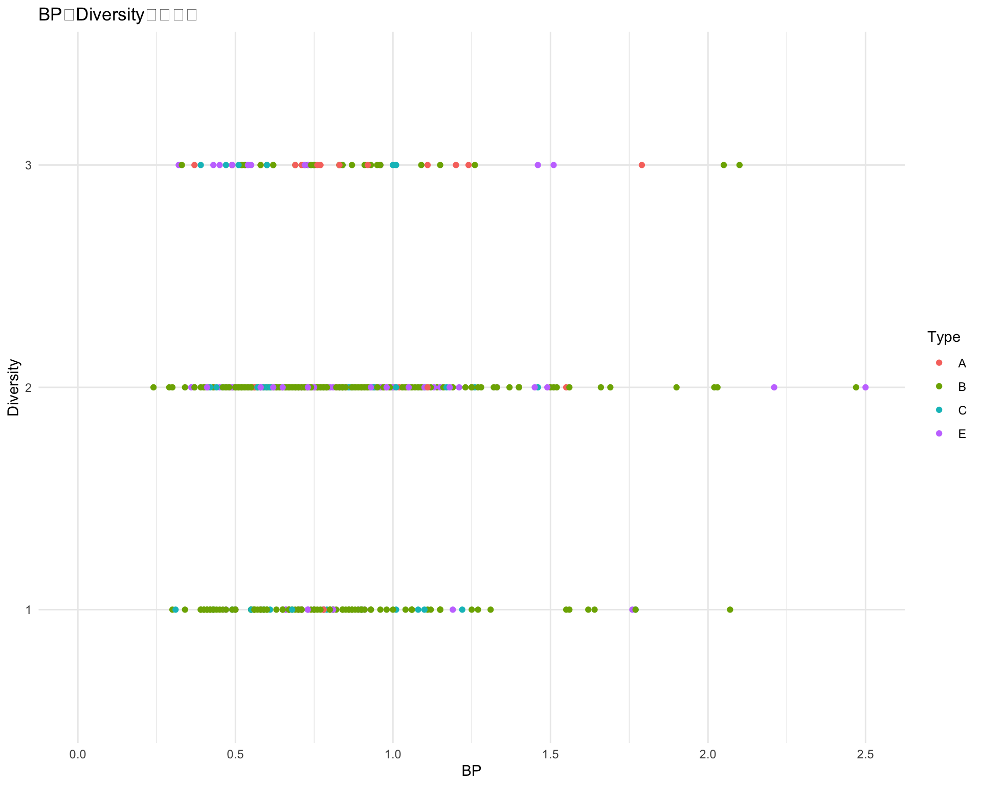
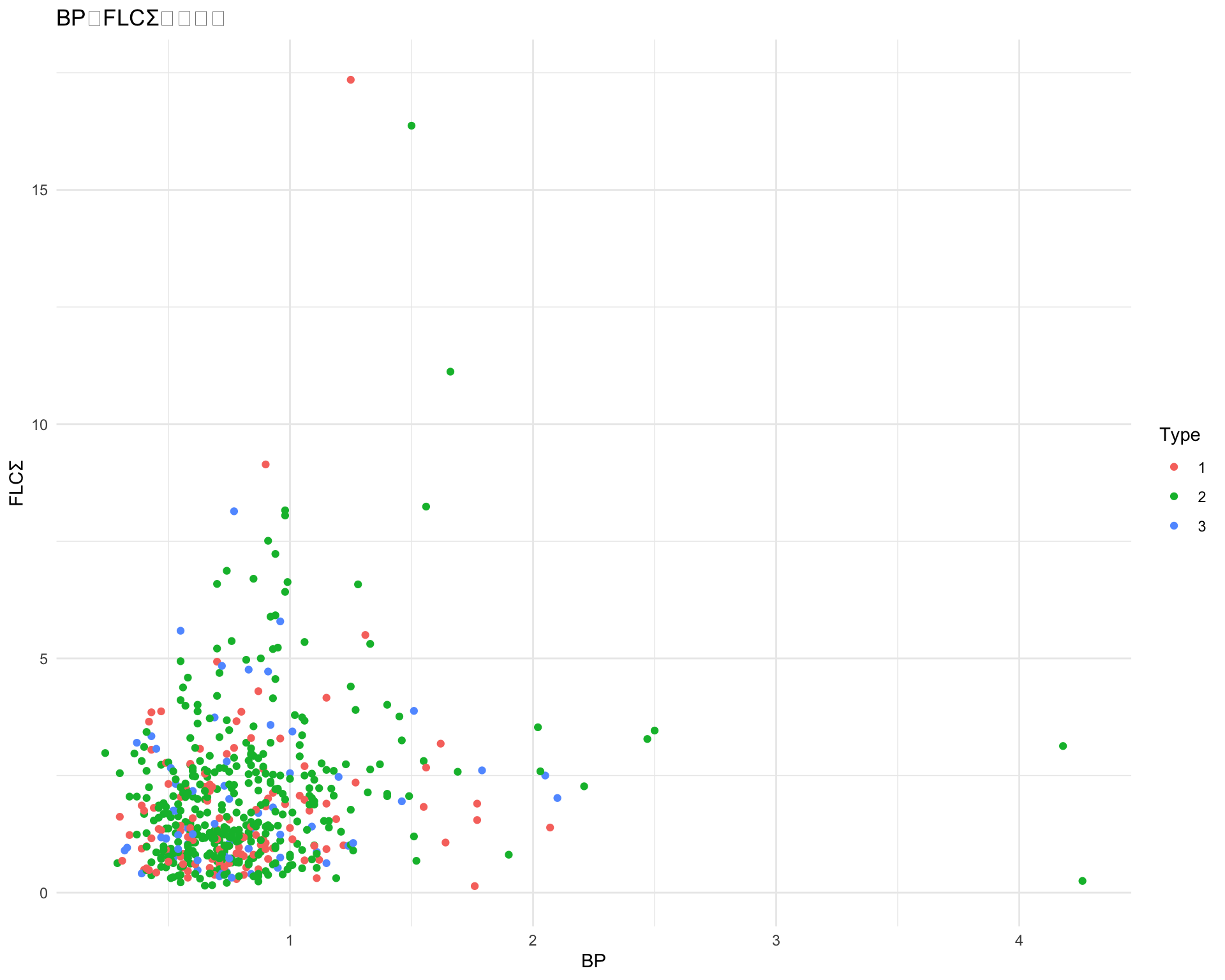
1.2 散布図

ggplot(df, aes(x = BP, y = diversity, color = type)) +
  geom_point() +
  labs(title = "BPとDiversityの散布図", x = "BP", y = "Diversity", color = "Type") +
  theme_minimal() +
  xlim(0, 2.5)
Warning: Removed 6 rows containing missing values (`geom_point()`).

ggplot(df, aes(x = BP, y = FLCΣ, color = type)) +
  geom_point() +
  labs(title = "BPとFLCΣの散布図", x = "BP", y = "FLCΣ", color = "Type") +
  theme_minimal()
Warning: Removed 4 rows containing missing values (`geom_point()`).

ggplot(df, aes(x = BP, y = FLCΣ, color = diversity)) +
  geom_point() +
  labs(title = "BPとFLCΣの散布図", x = "BP", y = "FLCΣ", color = "Type") +
  theme_minimal()
Warning: Removed 4 rows containing missing values (`geom_point()`).

1.3 BP の予測:全部切片にしてみる

library(brms)
bf <- bf(
  BP ~ 1 + (1|type:diversity)
)

fit_BP <- brm(
  formula = bf,
  data = df,
  family = gaussian(),
  iter = 8000, chains = 4, cores = 4)
ranef(fit_BP)$`type:diversity`
, , Intercept

        Estimate  Est.Error        Q2.5      Q97.5
A_1 -0.002120413 0.03894429 -0.09065862 0.07944242
A_2 -0.001433950 0.03269645 -0.07658970 0.06653257
A_3  0.013044669 0.03207317 -0.04176264 0.09221059
B_1 -0.024106006 0.02945986 -0.09479908 0.01749486
B_2 -0.002244259 0.02031005 -0.04846802 0.03739344
B_3 -0.012829030 0.03032269 -0.08715354 0.03901276
C_1  0.015190835 0.03484449 -0.04232356 0.10290872
C_2  0.013571711 0.03107443 -0.04034109 0.08951357
C_3  0.025477102 0.04294254 -0.03191079 0.13879133
E_1 -0.009731661 0.03469066 -0.09518904 0.05291874
E_2 -0.015391962 0.02768978 -0.08261422 0.02972215
E_3  0.003481505 0.03068718 -0.06071400 0.07271239
ranef <- ranef(fit_BP)$`type:diversity`
posterior_means <- ranef[,1,"Intercept"]
lower_bounds <- ranef[,3,"Intercept"]
upper_bounds <- ranef[,4,"Intercept"]
plot_df <- data.frame(
  type = rownames(ranef),
  mean = posterior_means,
  lower = lower_bounds,
  upper = upper_bounds
)
p <- ggplot(plot_df, aes(x = mean, y = type)) +
  geom_point() +
  geom_errorbar(aes(xmin = lower, xmax = upper), width = 0.2) +
  theme(axis.text.x = element_text(angle = 90, hjust = 1)) +
  labs(title = NULL,
       x = "Posterior Estimate",
       y = NULL)
p

1.4 BP の予測:多様性,ただしタイプごと

library(brms)
bf <- bf(
  BP ~ (type|diversity)
)

fit_BP_diversity <- brm(
  formula = bf,
  data = df,
  family = gaussian(),
  iter = 8000, chains = 4, cores = 4)
ranef(fit_BP_diversity)$diversity
, , Intercept

      Estimate  Est.Error       Q2.5     Q97.5
1 -0.031281118 0.09210050 -0.2862740 0.1280876
2 -0.021857364 0.09831240 -0.3137632 0.1408636
3  0.004603111 0.09274167 -0.2597889 0.1817238

, , typeB

       Estimate  Est.Error       Q2.5      Q97.5
1 -0.0297085922 0.05017291 -0.1433575 0.05872073
2  0.0004598164 0.03357642 -0.0759306 0.06762762
3 -0.0409713931 0.05463860 -0.1702725 0.03916893

, , typeC

    Estimate  Est.Error        Q2.5     Q97.5
1 0.07027170 0.08125771 -0.06041333 0.2464845
2 0.05212903 0.05838943 -0.05578777 0.1739574
3 0.11301646 0.09338545 -0.03577632 0.3123178

, , typeE

      Estimate  Est.Error       Q2.5      Q97.5
1 -0.016980625 0.05632744 -0.1580365 0.08526270
2 -0.020463399 0.03801587 -0.1136185 0.04382461
3 -0.004247138 0.04793339 -0.1149919 0.09507106
ranef <- ranef(fit_BP_diversity)$diversity
posterior_means <- ranef[,1,"Intercept"]
lower_bounds <- ranef[,3,"Intercept"]
upper_bounds <- ranef[,4,"Intercept"]
plot_df <- data.frame(
  diversity = rownames(ranef),
  mean = posterior_means,
  lower = lower_bounds,
  upper = upper_bounds
)
p <- ggplot(plot_df, aes(x = mean, y = diversity)) +
  geom_point() +
  geom_errorbar(aes(xmin = lower, xmax = upper), width = 0.2) +
  theme(axis.text.x = element_text(angle = 90, hjust = 1)) +
  labs(title = NULL,
       x = "Posterior Estimate",
       y = NULL)
p

2 個人の応答を予測できたら面白い

2.1 個人係数の予測

library(brms)
fit_1PL_cov <- readRDS("../../../Desktop/Mentalism/3-BayesianDataAnalysis/Cocosiru/rdb/fit_1PL_cov.rds")
ran_id_list <- ranef(fit_1PL_cov)$id[,1,]

df_IRT_long$ran_id <- ran_id_list[match(df_IRT_long$id, names(ran_id_list))]

df_IRT_long <- df_IRT_long[!is.na(df_IRT_long$ran_id), ]

summary(df_IRT_long$ran_id)
     Min.   1st Qu.    Median      Mean   3rd Qu.      Max. 
-1.765286 -0.880247 -0.790048 -0.002871  0.712761  3.994477 
library(brms)
bf <- bf(
  ran_id ~ 1 + (1|type)
)

fit_ranid <- brm(
  formula = bf,
  data = df_IRT_long,
  family = gaussian(),
  iter = 8000, chains = 4, cores = 4)
library(ggplot2)
ranef <- ranef(fit_ranid)$type
posterior_means <- ranef[,1,"Intercept"]
lower_bounds <- ranef[,3,"Intercept"]
upper_bounds <- ranef[,4,"Intercept"]
plot_df <- data.frame(
  type = rownames(ranef),
  mean = posterior_means,
  lower = lower_bounds,
  upper = upper_bounds
)
p <- ggplot(plot_df, aes(x = mean, y = type)) +
  geom_point() +
  geom_errorbar(aes(xmin = lower, xmax = upper), width = 0.2) +
  theme(axis.text.x = element_text(angle = 90, hjust = 1)) +
  labs(title = NULL,
       x = "Posterior Estimate",
       y = NULL)
p

2.2 タイプごとの係数の予測

大変重くて実行が難しい.

formula_1PL_cov <- bf(
  res ~ 1 + (1|item) + (BP|type) + FLCΣ
)
fit_1PL_cov_type <- brm(
  formula = formula_1PL_cov,
  data = df_IRT_long,
  family = brmsfamily("bernoulli", link = "logit"),
  iter = 8000, chains = 4, cores = 4
)
conditional_effects(fit_1PL_cov_type , effects = "FLCΣ")

ranefs <- ranef(fit_1PL_cov_type)$type
posterior_means <- ranefs[,1,"BP"]
lower_bounds <- ranefs[,3,"BP"]
upper_bounds <- ranefs[,4,"BP"]
plot_df <- data.frame(
  type = rownames(ranefs),
  mean = posterior_means,
  lower = lower_bounds,
  upper = upper_bounds
)

p <- ggplot(plot_df, aes(x = mean, y = type)) +
  geom_point() +
  geom_errorbar(aes(xmin = lower, xmax = upper), width = 0.2) +
  theme(axis.text.x = element_text(angle = 90, hjust = 1)) +
  labs(title = NULL,
       x = "Posterior Estimate",
       y = "Type") +
  theme(
    axis.text = element_text(size = 24),  # 軸の目盛りの文字サイズ
    axis.title = element_text(size = 30),   # 軸ラベルの文字サイズ
    legend.text = element_text(size = 36),  # 凡例のテキストサイズ
    legend.title = element_text(size = 24),  # 凡例のタイトルサイズ
    plot.margin = margin(r = 20, l = 10)  # 右側の余白を50ポイントに設定
  )
p

2.3 応答曲線は!?

ran_ef_list <- ranef(fit_1PL_cov_type)$item[,1,]
ran_coef0_list <- ranef(fit_1PL_cov_type)$type[,1,"Intercept"]
ran_coef1_list <- ranef(fit_1PL_cov_type)$type[,1,"BP"]

a <- -1.62
b <- -0.09

df_IRT_long$ran_ef <- ran_ef_list[match(df_IRT_long$item, names(ran_ef_list))]
df_IRT_long$ran_coef0 <- ran_coef0_list[match(df_IRT_long$type, names(ran_coef0_list))]
df_IRT_long$ran_coef1 <- ran_coef1_list[match(df_IRT_long$type, names(ran_coef1_list))]

df_IRT_long$pred_prob <- plogis(a + df_IRT_long$ran_ef + df_IRT_long$ran_coef0 + df_IRT_long$ran_coef1 * df_IRT_long$BP + b * df_IRT_long$FLCΣ)
library(pROC)
roc_obj <- roc(df_IRT_long$res, df_IRT_long$pred_prob)
plot(roc_obj)

roc_obj$auc
Area under the curve: 0.5997

2.4 くそ,もっと AUC 上がらないのか?

formula_type2 <- bf(
  res ~ 1 + (1|item) + (BP+FLCΣ|type)
)
fit_type2 <- brm(
  formula = formula_type2,
  data = df_IRT_long,
  family = brmsfamily("bernoulli", link = "logit"),
  iter = 8000, chains = 4, cores = 4
)
ranefs <- ranef(fit_type2)$type
posterior_means <- ranefs[,1,"BP"]
lower_bounds <- ranefs[,3,"BP"]
upper_bounds <- ranefs[,4,"BP"]
plot_df <- data.frame(
  type = rownames(ranefs),
  mean = posterior_means,
  lower = lower_bounds,
  upper = upper_bounds
)

p <- ggplot(plot_df, aes(x = mean, y = type)) +
  geom_point() +
  geom_errorbar(aes(xmin = lower, xmax = upper), width = 0.2) +
  theme(axis.text.x = element_text(angle = 90, hjust = 1)) +
  labs(title = NULL,
       x = "Posterior Estimate",
       y = "Type") +
  theme(
    axis.text = element_text(size = 24),  # 軸の目盛りの文字サイズ
    axis.title = element_text(size = 30),   # 軸ラベルの文字サイズ
    legend.text = element_text(size = 36),  # 凡例のテキストサイズ
    legend.title = element_text(size = 24),  # 凡例のタイトルサイズ
    plot.margin = margin(r = 20, l = 10)  # 右側の余白を50ポイントに設定
  )
p

ranefs <- ranef(fit_type2)$type
posterior_means <- ranefs[,1,"FLCΣ"]
lower_bounds <- ranefs[,3,"FLCΣ"]
upper_bounds <- ranefs[,4,"FLCΣ"]
plot_df <- data.frame(
  type = rownames(ranefs),
  mean = posterior_means,
  lower = lower_bounds,
  upper = upper_bounds
)

p <- ggplot(plot_df, aes(x = mean, y = type)) +
  geom_point() +
  geom_errorbar(aes(xmin = lower, xmax = upper), width = 0.2) +
  theme(axis.text.x = element_text(angle = 90, hjust = 1)) +
  labs(title = NULL,
       x = "Posterior Estimate",
       y = "Type") +
  theme(
    axis.text = element_text(size = 24),  # 軸の目盛りの文字サイズ
    axis.title = element_text(size = 30),   # 軸ラベルの文字サイズ
    legend.text = element_text(size = 36),  # 凡例のテキストサイズ
    legend.title = element_text(size = 24),  # 凡例のタイトルサイズ
    plot.margin = margin(r = 20, l = 10)  # 右側の余白を50ポイントに設定
  )
p

2.5 応答曲線上がれ!

ran_ef_list <- ranef(fit_type2)$item[,1,]
ran_coef0_list <- ranef(fit_type2)$type[,1,"Intercept"]
ran_coef1_list <- ranef(fit_type2)$type[,1,"BP"]
ran_coef2_list <- ranef(fit_type2)$type[,1,"FLCΣ"]

a <- -1.62

df_IRT_long$ran_ef <- ran_ef_list[match(df_IRT_long$item, names(ran_ef_list))]
df_IRT_long$ran_coef0 <- ran_coef0_list[match(df_IRT_long$type, names(ran_coef0_list))]
df_IRT_long$ran_coef1 <- ran_coef1_list[match(df_IRT_long$type, names(ran_coef1_list))]
df_IRT_long$ran_coef2 <- ran_coef2_list[match(df_IRT_long$type, names(ran_coef2_list))]

df_IRT_long$pred_prob <- plogis(a + df_IRT_long$ran_ef + df_IRT_long$ran_coef0 + df_IRT_long$ran_coef1 * df_IRT_long$BP + df_IRT_long$ran_coef2 * df_IRT_long$FLCΣ)
library(pROC)
roc_obj <- roc(df_IRT_long$res, df_IRT_long$pred_prob)
plot(roc_obj)

roc_obj$auc
Area under the curve: 0.6125

いや,上がることは上がるんだよな…….