library(brms)formula_2PL <-bf( res ~exp(loggamma) * eta, loggamma ~1+ (1|item), eta ~1+ (1|item) + (1|id),nl =TRUE)fit_2PL <-brm(formula = formula_2PL,data = df_1PL_long,family =brmsfamily("bernoulli", link ="logit"),chains =4, cores =4, iter =5000)
1.3 1PL モデル
library(brms)
Warning: パッケージ 'brms' はバージョン 4.3.1 の R の下で造られました
要求されたパッケージ Rcpp をロード中です
Loading 'brms' package (version 2.21.0). Useful instructions
can be found by typing help('brms'). A more detailed introduction
to the package is available through vignette('brms_overview').
次のパッケージを付け加えます: 'brms'
 以下のオブジェクトは 'package:stats' からマスクされています:

    ar
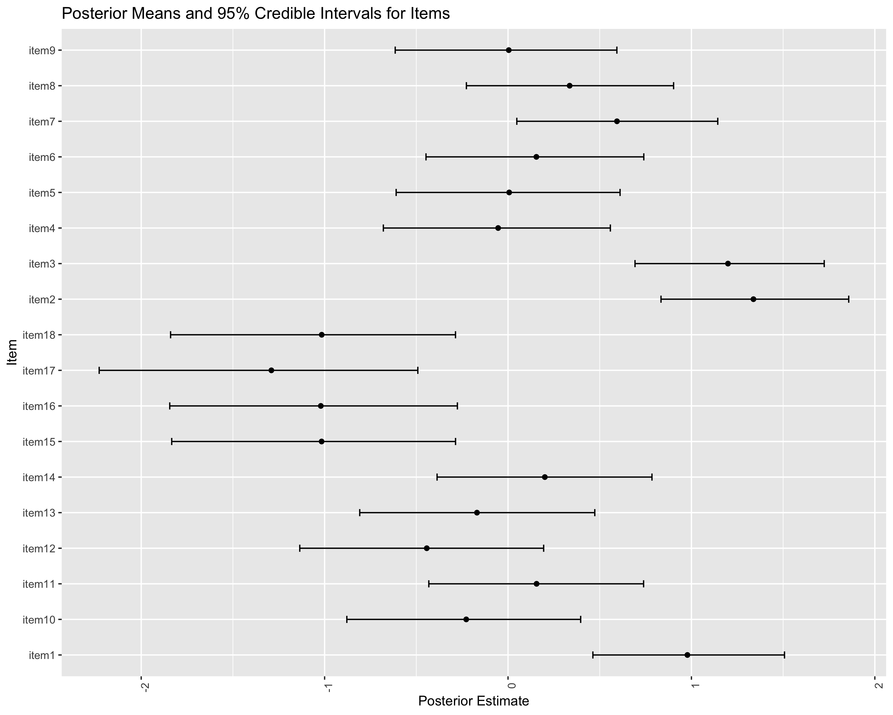
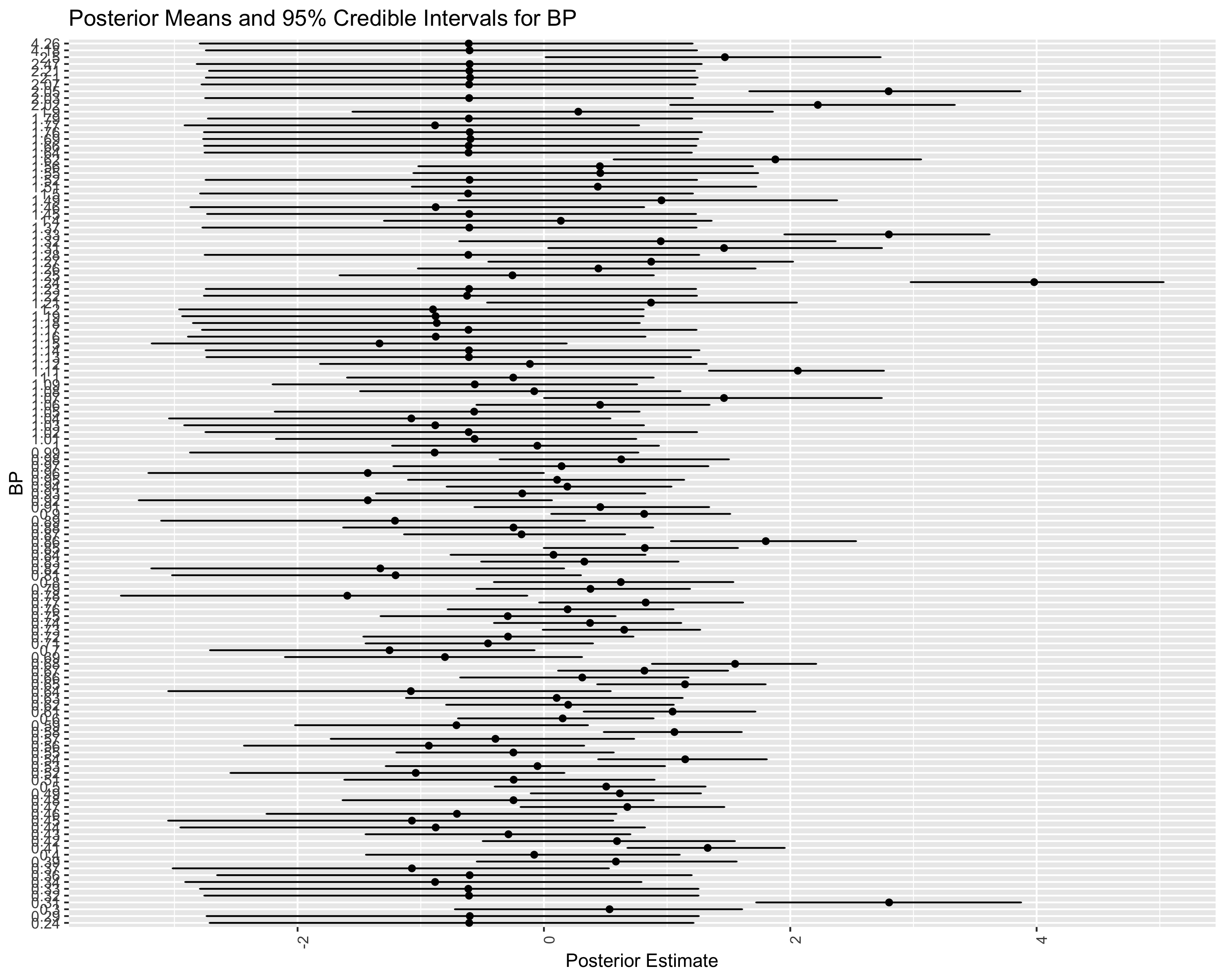
formula_1PL <-bf( res ~1+ (1|item) + (1|BP))fit_1PL <-brm(formula = formula_1PL,data = df_1PL_long,family =brmsfamily("bernoulli", link ="logit"),chains =4, cores =4, iter =5000)
Warning: Rows containing NAs were excluded from the model.
Compiling Stan program...
Start sampling
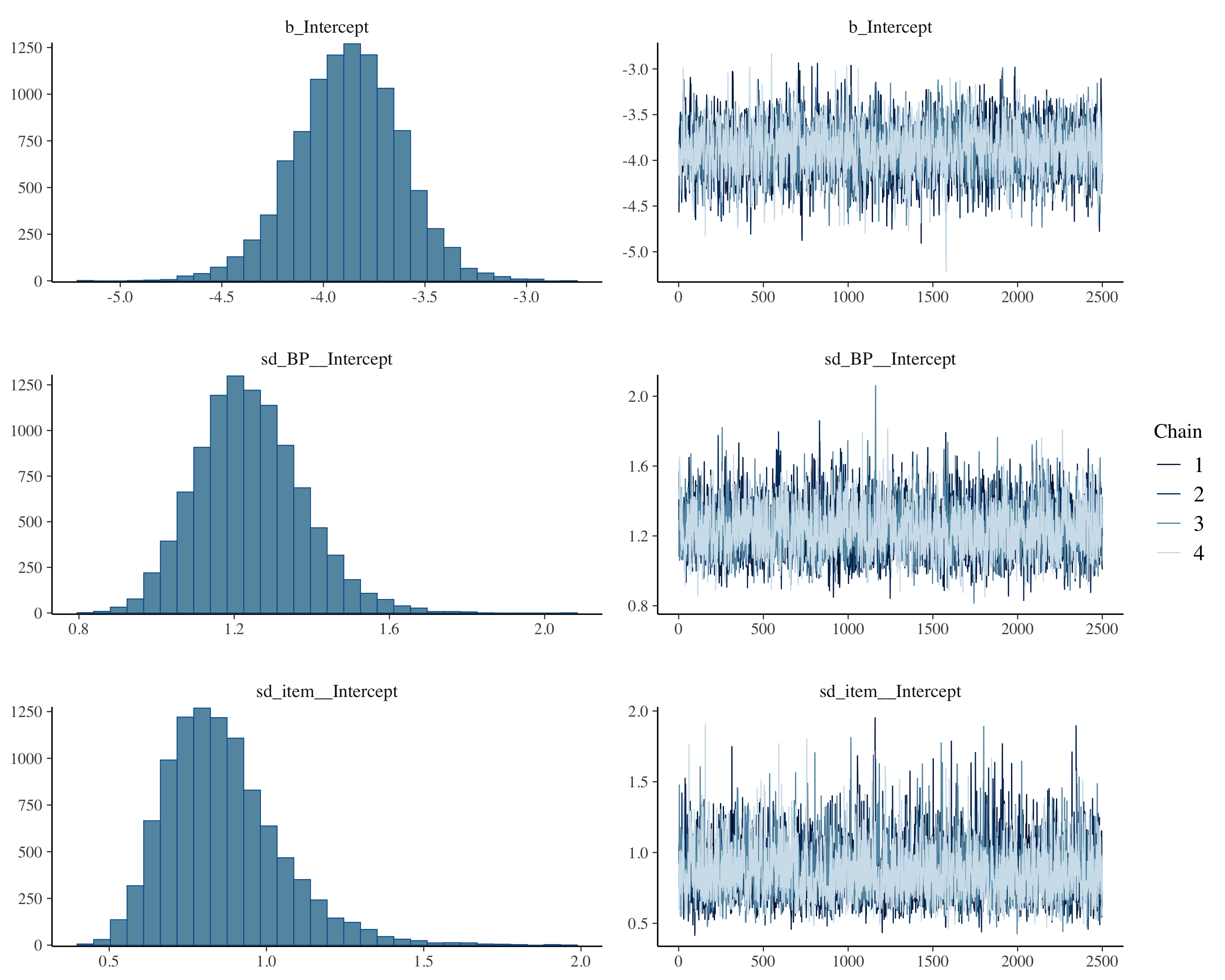
summary(fit_1PL)
 Family: bernoulli
  Links: mu = logit
Formula: res ~ 1 + (1 | item) + (1 | BP)
   Data: df_1PL_long (Number of observations: 10365)
  Draws: 4 chains, each with iter = 5000; warmup = 2500; thin = 1;
         total post-warmup draws = 10000

Multilevel Hyperparameters:
~BP (Number of levels: 130)
              Estimate Est.Error l-95% CI u-95% CI Rhat Bulk_ESS Tail_ESS
sd(Intercept)     1.24      0.14     0.99     1.54 1.00     3054     4847

~item (Number of levels: 18)
              Estimate Est.Error l-95% CI u-95% CI Rhat Bulk_ESS Tail_ESS
sd(Intercept)     0.86      0.18     0.57     1.30 1.00     3752     5935

Regression Coefficients:
          Estimate Est.Error l-95% CI u-95% CI Rhat Bulk_ESS Tail_ESS
Intercept    -3.88      0.26    -4.41    -3.37 1.00     2903     4664

Draws were sampled using sampling(NUTS). For each parameter, Bulk_ESS
and Tail_ESS are effective sample size measures, and Rhat is the potential
scale reduction factor on split chains (at convergence, Rhat = 1).