弘前データ解析１-６：BP のみによる予測

ARMS バイオマーカーは質問表応答も予測するか？

著者

司馬博文

日付

6/25/2025

Modified

6/25/2025

はじめに

hirosaki1-3.qmd では BP と \(\Sigma\)-FLC が高いほど項目応答確率が上がることを見た．しかしこれは先行研究 (Wake et al., 2022) と食い違う．2×2 で見たり，交差項を考えたりすることで，この構造をさらに詳しくみる．

元論文のロジスティック解析では，（クレアチン補正した）BP と \(\Sigma\)-FLC の値を正規化せず，そのままのスケールを保つことで discrimination score を構成し，これを cut-off value \(-0.096\) で２値判別することで，AUC \(0.912\) を達成している．

1 導入

1.1 備考データの除去

\(\Sigma\)-FLC の備考データも取り除く．

library(readxl)
library(knitr)
df <- readRDS("df.rds")
df <- df[is.na(df$`BP備考`), ]
dim(df)

[1] 584  22

kable(head(df))

	id	age	sex	Weight	BP	FLCΣ	BP備考	判別式	LOX	LAB	LOX_Index	type	diversity	BMI	med	med_col	年代	活気	イライラ感	疲労感	不安感	抑うつ感
3	4	46	1	76.3	1.10	1.95	NA	-2.974	136	3.8	517	B	2	26.0	2	NA	40代	2	3	2	3	2
5	6	30	1	59.5	0.76	0.64	NA	-2.776	46	2.2	101	B	2	19.5	2	NA	30代	3	5	4	5	4
6	7	51	1	76.6	1.69	2.58	NA	-2.377	78	3.2	250	B	2	25.5	2	NA	50代	3	3	3	3	2
7	8	47	2	43.2	0.56	0.55	NA	-3.048	40	2.7	108	B	2	16.7	2	NA	40代	2	1	2	2	1
9	10	39	1	61.9	0.52	0.64	NA	-3.165	54	2.4	130	B	2	21.3	2	NA	30代	3	3	3	3	3
10	11	55	1	61.0	0.89	2.64	NA	-3.708	60	3.1	186	E	1	22.9	1	NA	50代	3	2	2	1	1

に対して長形式のデータは次の通り：

df_IRT_long <- readRDS("df_IRT_long.rds")
df_IRT_long <- df_IRT_long[df_IRT_long$FLCΣ > 0, ]
kable(head(df_IRT_long))

	id	BP	FLCΣ	type	diversity	item	response	res
1	2	0.47	0.81	B	2	活気	3	0
2	2	0.47	0.81	B	2	イライラ感	3	0
3	2	0.47	0.81	B	2	疲労感	4	1
4	2	0.47	0.81	B	2	不安感	3	0
5	2	0.47	0.81	B	2	抑うつ感	3	0
11	4	1.10	1.95	B	2	活気	2	0

2 BP のみによる予測

library(brms)
formula <- bf(
  res ~ 1 + (1 | item) + (1 | id) + BP
)
prior_1PL <-  prior("normal(0,3)", class="sd", group = "id") + prior("normal(0,3)", class="sd", group = "item")
fit_1PL <- brm(
  formula = formula,
  data = df_IRT_long,
  family = brmsfamily("bernoulli", link = "logit"),
  prior = prior_1PL,
  chains = 4, cores = 4, iter = 8000
)

2.1 後知恵判別分析の実行

ran_ef_list <- ranef(fit_1PL)$item[,1,]
ran_id_list <- ranef(fit_1PL)$id[,1,]

df_IRT_long$ran_ef <- ran_ef_list[match(df_IRT_long$item, names(ran_ef_list))]
df_IRT_long$ran_id <- ran_id_list[match(df_IRT_long$id, names(ran_id_list))]

beta_0 <- -2.97
beta_BP <- 0.32

df_IRT_long$discrimination_score <- beta_0 + beta_BP * df_IRT_long$BP + df_IRT_long$ran_ef + df_IRT_long$ran_id

df_IRT_long <- df_IRT_long[!is.na(df_IRT_long$discrimination_score),]

summary(df_IRT_long$discrimination_score)

   Min. 1st Qu.  Median    Mean 3rd Qu.    Max. 
 -4.099  -3.726  -3.040  -2.755  -2.035   2.013

param <- seq(-4.1, 2.05, 0.001)
x <- c()
y <- c()

for (threshold in param) {
  res_predicted <- df_IRT_long$discrimination_score > threshold

  is_false <- res_predicted != df_IRT_long$res
  is_true <- res_predicted == df_IRT_long$res
  
  x <- append(x, mean(is_false[df_IRT_long$res == 0], na.rm = TRUE))
  y <- append(y, mean(is_true[df_IRT_long$res == 1], na.rm = TRUE))
}

library(ggplot2)

ggplot(data.frame(x = x, y = y), aes(x = x, y = y)) +
  geom_point(size = 2) +
  geom_line() +
  theme_minimal() +
  labs(x = "False Positive Rate", y = "True Positive Rate") +
  lims(x = c(0, 1), y = c(0, 1))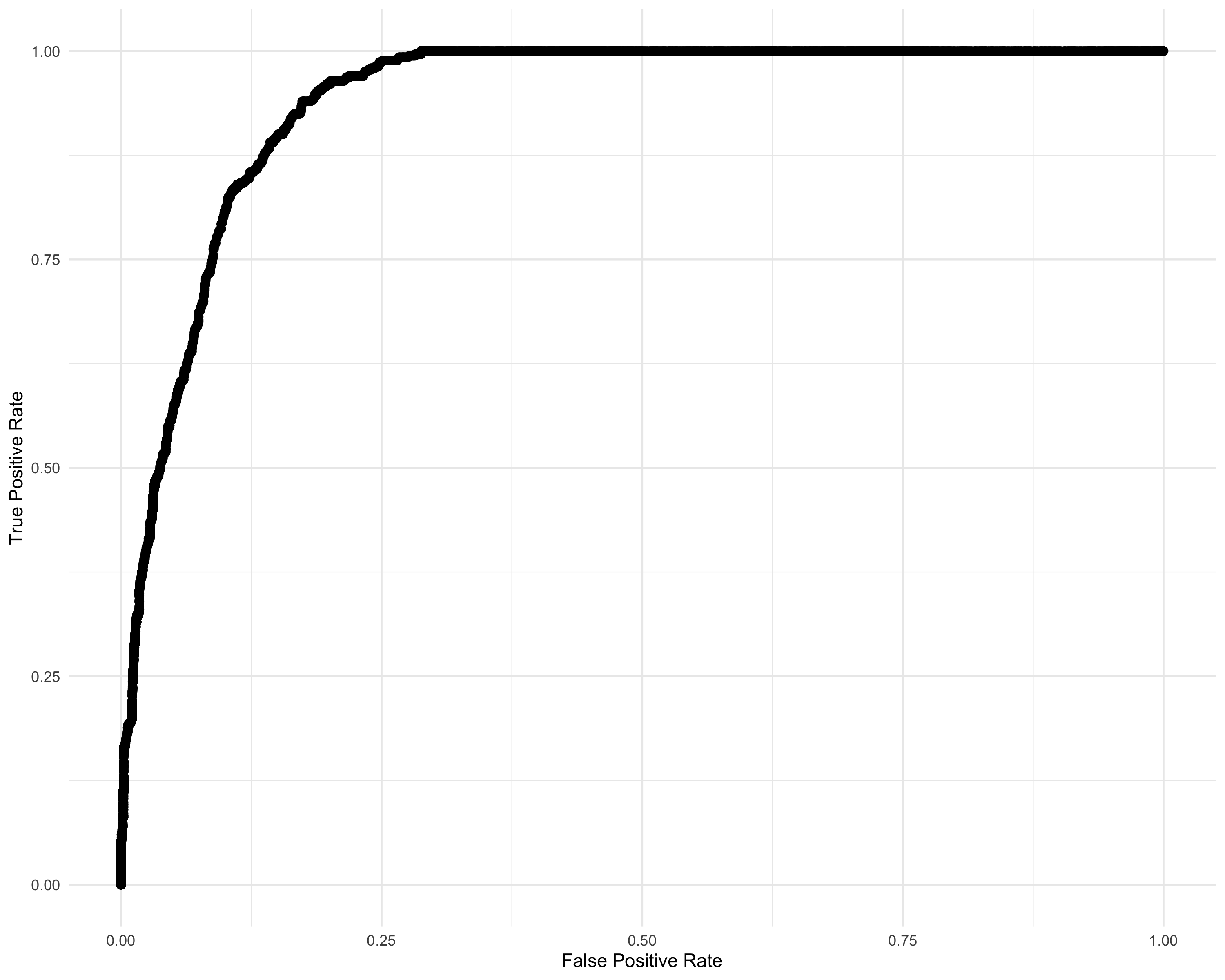

logistic <- function(x) {
  return(1 / (1 + exp(-x)))
}

library(dplyr)


 次のパッケージを付け加えます: 'dplyr'

 以下のオブジェクトは 'package:stats' からマスクされています:

    filter, lag

 以下のオブジェクトは 'package:base' からマスクされています:

    intersect, setdiff, setequal, union

df_IRT_long <- df_IRT_long %>%
  mutate(prediction = logistic(discrimination_score))

library(pROC)

Warning: パッケージ 'pROC' はバージョン 4.3.3 の R の下で造られました

Type 'citation("pROC")' for a citation.


 次のパッケージを付け加えます: 'pROC'

 以下のオブジェクトは 'package:stats' からマスクされています:

    cov, smooth, var

roc_obj <- roc(response = df_IRT_long$res, predictor = df_IRT_long$prediction)

Setting levels: control = 0, case = 1

Setting direction: controls < cases

plot(roc_obj)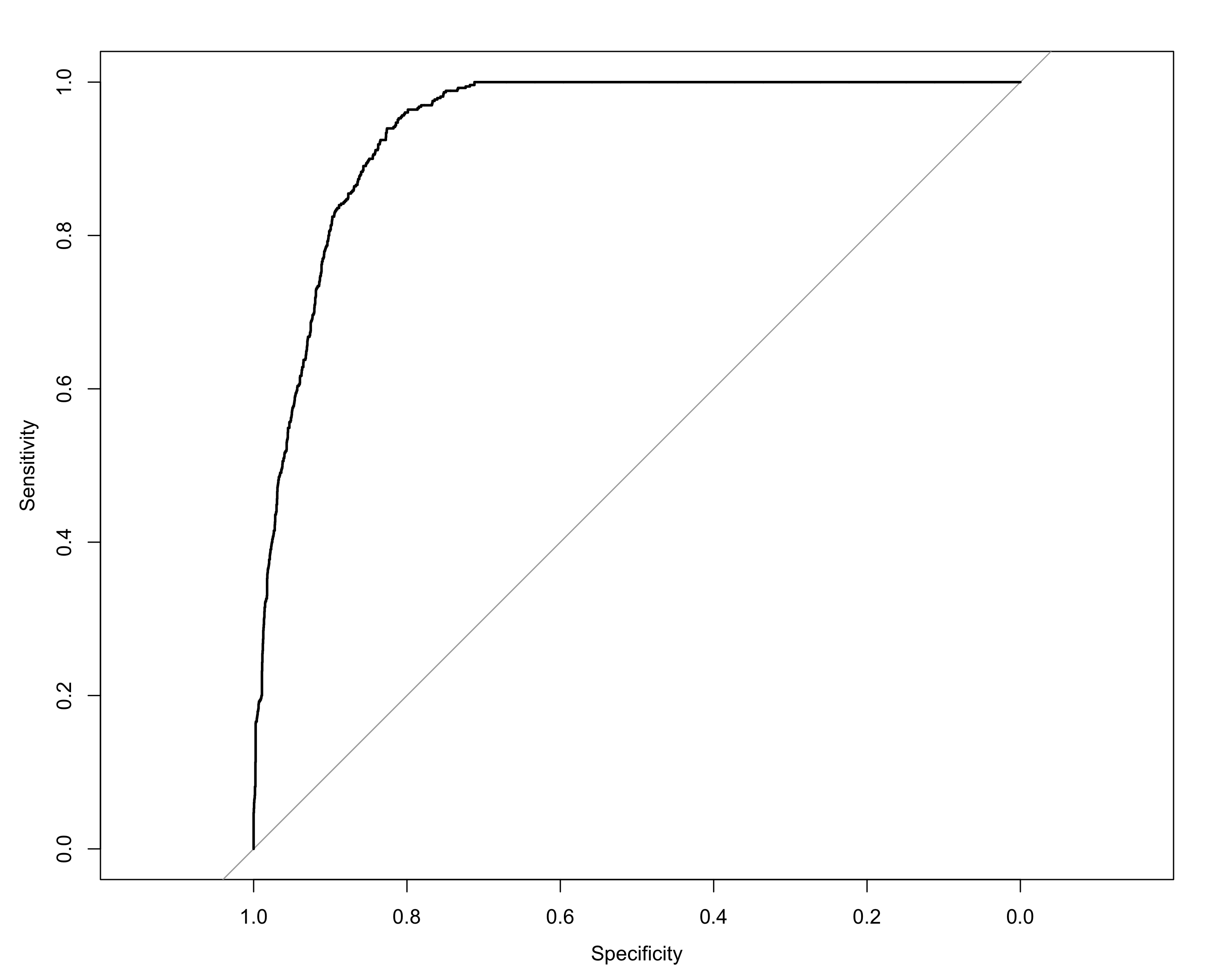

auc(roc_obj)

Area under the curve: 0.9409

2.2 個人ごとの係数を見てみよう

library(ggplot2)
ranef_id <- ranef(fit_1PL)$id
posterior_means <- ranef_id[,1,1]
lower_bounds <- ranef_id[,3,1]
upper_bounds <- ranef_id[,4,1]
plot_df_id <- data.frame(
  id = rownames(ranef_id),
  mean = posterior_means,
  lower = lower_bounds,
  upper = upper_bounds
)

plot_df_id <- plot_df_id %>% arrange(mean) %>% mutate(rank = row_number())
p_PL1_id <- ggplot(plot_df_id, aes(x = mean, y = rank)) +
  geom_point() +
  geom_errorbar(aes(xmin = lower, xmax = upper), width = 0.2) +
  theme(
    axis.text = element_text(size = 24),  # 軸の目盛りの文字サイズ
    axis.title = element_text(size = 30),   # 軸ラベルの文字サイズ
    legend.text = element_text(size = 36),  # 凡例のテキストサイズ
    legend.title = element_text(size = 24),  # 凡例のタイトルサイズ
    # plot.margin = margin(r = 20)  # 右側の余白を50ポイントに設定
  ) +
  labs(title = "Posterior Means and 95% Credible Intervals for Individuals",
       x = "b",
       y = "Individual (ID)")
p_PL1_id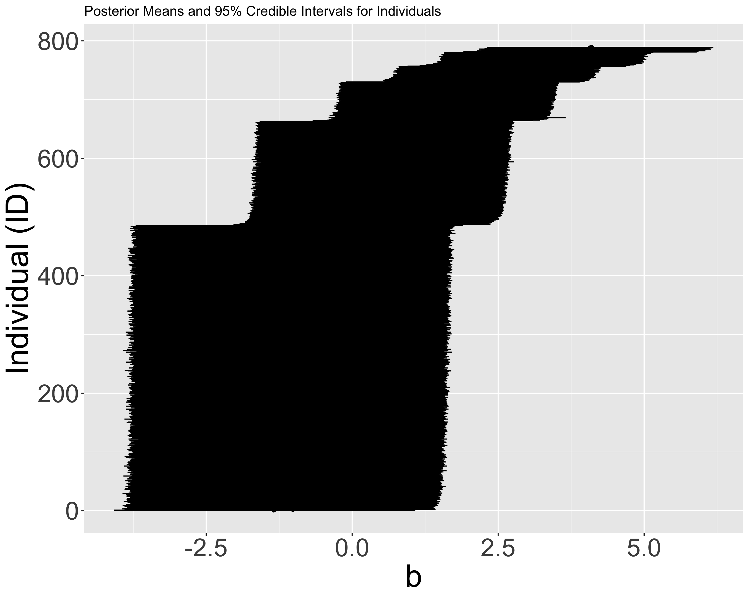

クラスタリングするだけでも精度が出そうだな．

References

Wake, R., Araki, T., Fukushima, M., Matsuda, H., Inagaki, T., Hayashida, M., … Oh-Nishi, A. (2022). Urinary biopyrrins and free immunoglobin light chains are biomarker candidates for screening at-risk mental state in adolescents. Early Intervention in Psychiatry, 16(3), 272–280.