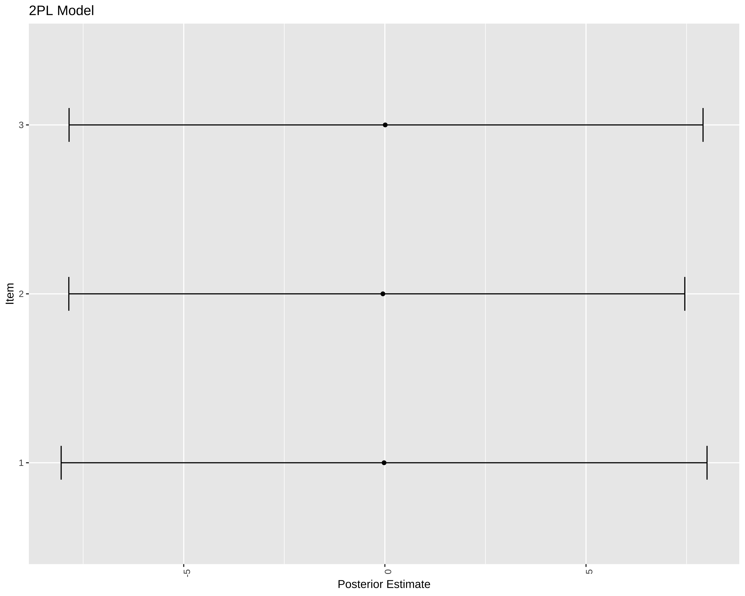
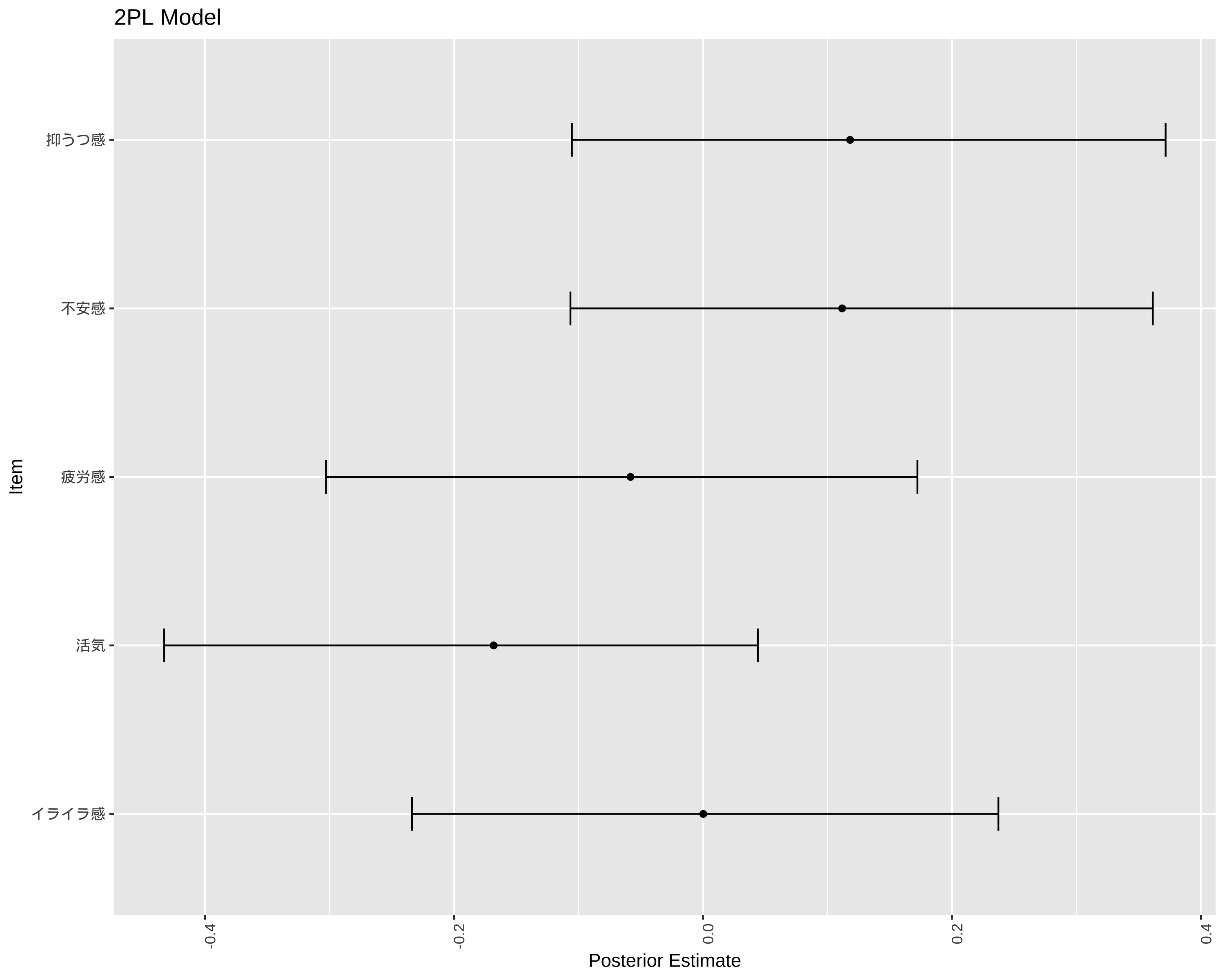
弘前データ１-３：法定検診との関係の詳細検討

BP の値の高低を用いた項目反応モデル＋変動係数を追加した線型回帰モデル

はじめに

前々稿では BP, FLCΣ の値で３段階に離散化・層別して可視化した． ここでは層別して回帰する，項目反応モデリングを考える． 項目毎・個人毎のパラメータを識別するのはうまくいかないことを前稿で見たから，ここでは「活気」「抑うつ感」のレベルで，そして BP のレベル感３クラスで，別々のパラメータを推定することを考える．さらに，「４以上の値を取る」という事象のみに向かって回帰する．

最後に，項目毎の固定効果と個人毎の固定効果を追加することで過分散を吸収し，その下で BP と \(\Sigma\)-FLC の効果を見た．すると綺麗な条件付き効果のプロットを得ることができる．

kable(head(df))

受付番号	受診日年齢	性別	Weight	BP	FLCΣ	BP備考	判別式	LOX-1_H	LAB_H	LOX-index_H	タイプ	多様性	item1	item2	item3	item4	item5	item6	item7	item8	item9	item10	item11	item12	item13	item14	item15	item16	item17	item18	年代	活気	イライラ感	疲労感	不安感	抑うつ感
4	46	1	76.3	1.10	1.95	NA	-2.974	136	3.8	517	B	2	2	3	3	2	2	2	1	1	2	2	2	1	2	2	1	1	1	1	40代	2	3	2	3	2
6	30	1	59.5	0.76	0.64	NA	-2.776	46	2.2	101	B	2	2	2	2	3	4	3	3	3	3	4	4	3	3	3	3	3	1	1	30代	3	5	4	5	4
7	51	1	76.6	1.69	2.58	NA	-2.377	78	3.2	250	B	2	2	2	2	2	2	2	2	2	2	2	2	2	2	1	1	1	1	1	50代	3	3	3	3	2
8	47	2	43.2	0.56	0.55	NA	-3.048	40	2.7	108	B	2	3	3	3	1	1	1	2	1	1	2	1	1	1	1	1	1	1	1	40代	2	1	2	2	1
10	39	1	61.9	0.52	0.64	NA	-3.165	54	2.4	130	B	2	2	2	2	2	2	2	2	2	2	2	2	2	2	2	2	2	2	2	30代	3	3	3	3	3
11	55	1	61.0	0.89	2.64	NA	-3.708	60	3.1	186	E	1	2	2	2	1	1	2	1	1	2	1	1	1	1	1	1	1	1	1	50代	3	2	2	1	1

1 低解像度項目反応モデル

1.1 データ長形式化

df_IRT <- df[, c("受付番号", "BP", "FLCΣ", "活気", "イライラ感", "疲労感", "不安感", "抑うつ感")]
colnames(df_IRT)[1] <- "id"

library(tidyr)

df_IRT_long <- df_IRT %>%
  pivot_longer(
    cols = c("活気", "イライラ感", "疲労感", "不安感", "抑うつ感"),
    names_to = "item",
    values_to = "response"
)

df_IRT_long$res <- ifelse(df_IRT_long$response > 3, 1, 0)

kable(head(df_IRT_long[6:13,]))

id	BP	FLCΣ	item	response	res
6	0.76	0.64	活気	3	0
6	0.76	0.64	イライラ感	5	1
6	0.76	0.64	疲労感	4	1
6	0.76	0.64	不安感	5	1
6	0.76	0.64	抑うつ感	4	1
7	1.69	2.58	活気	3	0

1.2 BP_level の設定

df_IRT_long$BP_level <- case_when(
  df_IRT_long$BP > 0.9 ~ 3,
  df_IRT_long$BP > 0.7 & df_IRT_long$BP <= 0.9 ~ 2,
  df_IRT_long$BP <= 0.7 ~ 1
)
length(df_IRT_long[df_IRT_long$BP_level == 3, ]$BP)/dim(df_IRT_long)[1]

[1] 0.2945205

length(df_IRT_long[df_IRT_long$BP_level == 2, ]$BP)/dim(df_IRT_long)[1]

[1] 0.2962329

length(df_IRT_long[df_IRT_long$BP_level == 1, ]$BP)/dim(df_IRT_long)[1]

[1] 0.4366438

1.3 2PL モデル

\[ g(\operatorname{P}[Y_{ij}=1])=\gamma_j\bigg(\alpha_j+\beta_i\bigg) \]

library(brms)

formula_2PL <- bf(
  res ~ exp(loggamma) * eta,
  loggamma ~ 1 + (1|item),
  eta ~ 1 + (1|item) + (1|BP_level),
  nl = TRUE
)

fit_2PL <- brm(
  formula = formula_2PL,
  data = df_IRT_long,
  family = brmsfamily("bernoulli", link = "logit"),
  chains = 4, cores = 4, iter = 8000
)
saveRDS(fit_2PL, "fit_2PL.rds")

Warning: パッケージ 'brms' はバージョン 4.3.1 の R の下で造られました

 要求されたパッケージ Rcpp をロード中です 

Loading 'brms' package (version 2.21.0). Useful instructions
can be found by typing help('brms'). A more detailed introduction
to the package is available through vignette('brms_overview').

 次のパッケージを付け加えます: 'brms' 

 以下のオブジェクトは 'package:stats' からマスクされています:

    ar

1.4 結果のプロット

\(\eta\) の存在感が消えてしまう，識別力パラメータで全てを説明し切ってしまう．

1.4.1 項目母数 \(\alpha_j\)

library(ggplot2)
library(gridExtra)

 次のパッケージを付け加えます: 'gridExtra' 

 以下のオブジェクトは 'package:dplyr' からマスクされています:

    combine

library(showtext)  # 日本語フォント用のパッケージ

 要求されたパッケージ sysfonts をロード中です 

 要求されたパッケージ showtextdb をロード中です 

# 日本語フォントの設定
font_add_google("Noto Sans JP", "notosans")  # Google Fontsからフォントを追加
showtext_auto()  # 自動的にshowtextを使用するように設定

ranef_item2 <- ranef(fit_2PL)$item
posterior_means <- ranef_item2[,1,"eta_Intercept"]
lower_bounds <- ranef_item2[,3,"eta_Intercept"]
upper_bounds <- ranef_item2[,4,"eta_Intercept"]
plot_df_item2 <- data.frame(
  item = rownames(ranef_item2),
  mean = posterior_means,
  lower = lower_bounds,
  upper = upper_bounds
)
p_PL2 <- ggplot(plot_df_item2, aes(x = mean, y = item)) +
  geom_point() +
  geom_errorbar(aes(xmin = lower, xmax = upper), width = 0.2) +
  theme(axis.text.x = element_text(angle = 90, hjust = 1)) +
  labs(title = NULL,
       x = "Posterior Estimate",
       y = NULL)
p_PL2

1.4.2 識別力母数 \(\gamma_j\)

ranef_item2 <- ranef(fit_2PL)$item
posterior_means <- ranef_item2[,1,"loggamma_Intercept"]
lower_bounds <- ranef_item2[,3,"loggamma_Intercept"]
upper_bounds <- ranef_item2[,4,"loggamma_Intercept"]
plot_df_item2 <- data.frame(
  item = rownames(ranef_item2),
  mean = posterior_means,
  lower = lower_bounds,
  upper = upper_bounds
)
p_PL2 <- ggplot(plot_df_item2, aes(x = mean, y = item)) +
  geom_point() +
  geom_errorbar(aes(xmin = lower, xmax = upper), width = 0.2) +
  theme(axis.text.x = element_text(angle = 90, hjust = 1)) +
  labs(title = NULL,
       x = "Posterior Estimate",
       y = NULL) +
   theme(
    axis.text = element_text(size = 24),  # 軸の目盛りの文字サイズ
    axis.title = element_text(size = 30),   # 軸ラベルの文字サイズ
    legend.text = element_text(size = 36),  # 凡例のテキストサイズ
    legend.title = element_text(size = 24),  # 凡例のタイトルサイズ
    plot.margin = margin(r = 20)  # 右側の余白を50ポイントに設定
  )
p_PL2

識別力パラメータを見ることで，「不安感」と「抑うつ感」だけ BP に関係していることが見えてくる．

1.4.3 個人母数 \(\beta_i\)

ranef_BP_level <- ranef(fit_2PL)$BP_level
posterior_means <- ranef_BP_level[,1,"eta_Intercept"]
lower_bounds <- ranef_BP_level[,3,"eta_Intercept"]
upper_bounds <- ranef_BP_level[,4,"eta_Intercept"]
plot_df_BP_level <- data.frame(
  BP_level = rownames(ranef_BP_level),
  mean = posterior_means,
  lower = lower_bounds,
  upper = upper_bounds
)
p_PL2 <- ggplot(plot_df_BP_level, aes(x = mean, y = BP_level)) +
  geom_point() +
  geom_errorbar(aes(xmin = lower, xmax = upper), width = 0.2) +
  theme(axis.text.x = element_text(angle = 90, hjust = 1)) +
  labs(title = "2PL Model",
       x = "Posterior Estimate",
       y = "Item")
p_PL2

1.5 1PL モデル

\[ g(\operatorname{P}[Y_{ij}=1])=\alpha_j+\beta_i \]

library(brms)

formula_1PL <- bf(
  res ~ 1 + (1|item) + (1|BP_level)
)

fit_1PL <- brm(
  formula = formula_1PL,
  data = df_IRT_long,
  family = brmsfamily("bernoulli", link = "logit"),
  chains = 4, cores = 4, iter = 8000
)
saveRDS(fit_1PL, "fit_1PL.rds")

library(ggplot2)
ranef_item <- ranef(fit_1PL)$item
posterior_means <- ranef_item[,1,1]
lower_bounds <- ranef_item[,3,1]
upper_bounds <- ranef_item[,4,1]
plot_df_item <- data.frame(
  item = rownames(ranef_item),
  mean = posterior_means,
  lower = lower_bounds,
  upper = upper_bounds
)
p_PL1 <- ggplot(plot_df_item, aes(x = mean, y = item)) +
  geom_point() +
  geom_errorbar(aes(xmin = lower, xmax = upper), width = 0.2) +
  theme(axis.text.x = element_text(angle = 90, hjust = 1)) +
  labs(title = "Posterior Means and 95% Credible Intervals for Items",
       x = "Posterior Estimate",
       y = "Item")
p_PL1

ranef_BP_level <- ranef(fit_1PL)$BP_level
posterior_means <- ranef_BP_level[,1,1]
lower_bounds <- ranef_BP_level[,3,1]
upper_bounds <- ranef_BP_level[,4,1]
plot_df_BP_level <- data.frame(
  BP_level = rownames(ranef_BP_level),
  mean = posterior_means,
  lower = lower_bounds,
  upper = upper_bounds
)

plot_df_BP_level <- plot_df_BP_level %>% arrange(mean) %>% mutate(rank = row_number())
p_PL1_BP_level <- ggplot(plot_df_BP_level, aes(x = mean, y = rank)) +
  geom_point() +
  geom_errorbar(aes(xmin = lower, xmax = upper), width = 0.2) +
  theme(axis.text.x = element_text(angle = 90, hjust = 1)) +
  labs(title = NULL,
       x = "Posterior Estimate",
       y = "BP Level") +
   theme(
    axis.text = element_text(size = 24),  # 軸の目盛りの文字サイズ
    axis.title = element_text(size = 30),   # 軸ラベルの文字サイズ
    legend.text = element_text(size = 36),  # 凡例のテキストサイズ
    legend.title = element_text(size = 24),  # 凡例のタイトルサイズ
    plot.margin = margin(r = 20, l = 10)  # 右側の余白を50ポイントに設定
  )
p_PL1_BP_level

確かに，BP レベルが高い人ほど，全般的に回答に高い点数（4や5）を付けやすいことは見て取れる．

2 FLC で同じことをやる

2.1 FLC の層別

次のように，30%, 30%, 40% に分ける．

library(dplyr)
df_IRT_long$FLC_level <- case_when(
  df_IRT_long$FLCΣ >= 2 ~ 3,
  df_IRT_long$FLCΣ >= 1.0 & df_IRT_long$FLCΣ < 2 ~ 2,
  df_IRT_long$FLCΣ < 1.0 ~ 1
)
length(df_IRT_long[df_IRT_long$FLC_level == 3, ]$FLCΣ)/dim(df_IRT_long)[1]

[1] 0.390411

length(df_IRT_long[df_IRT_long$FLC_level == 2, ]$FLCΣ)/dim(df_IRT_long)[1]

[1] 0.3219178

length(df_IRT_long[df_IRT_long$FLC_level == 1, ]$FLCΣ)/dim(df_IRT_long)[1]

[1] 0.3150685

2.2 2PL モデル

なぜかとてもサンプリングが遅い！構造がそんなにも違うのか！

library(brms)

formula_2PL <- bf(
  res ~ exp(loggamma) * eta,
  loggamma ~ 1 + (1|item),
  eta ~ 1 + (1|item) + (1|FLC_level),
  nl = TRUE
)

FLC_2PL <- brm(
  formula = formula_2PL,
  data = df_IRT_long,
  family = brmsfamily("bernoulli", link = "logit"),
  chains = 4, cores = 4, iter = 8000
)

saveRDS(FLC_2PL, "./1-3/FLC_2PL.rds")

2.2.1 識別力パラメータ

基本的に BP と同じになる．計算が長すぎるので省略する．

ranef_item_FLC <- ranef(FLC_2PL)$item
posterior_means <- ranef_item_FLC[,1,"loggamma_Intercept"]
lower_bounds <- ranef_item_FLC[,3,"loggamma_Intercept"]
upper_bounds <- ranef_item_FLC[,4,"loggamma_Intercept"]
plot_df_item_FLC <- data.frame(
  item = rownames(ranef_item_FLC),
  mean = posterior_means,
  lower = lower_bounds,
  upper = upper_bounds
)
p_PL2_FLC <- ggplot(plot_df_item_FLC, aes(x = mean, y = item)) +
  geom_point() +
  geom_errorbar(aes(xmin = lower, xmax = upper), width = 0.2) +
  theme(axis.text.x = element_text(angle = 90, hjust = 1)) +
  labs(title = "2PL Model",
       x = "Posterior Estimate",
       y = "Item")
p_PL2_FLC

2.3 1PL モデル

library(brms)

formula_1PL <- bf(
  res ~ 1 + (1|item) + (1|FLC_level)
)

FLC_1PL <- brm(
  formula = formula_1PL,
  data = df_IRT_long,
  family = brmsfamily("bernoulli", link = "logit"),
  chains = 4, cores = 4, iter = 8000
)
saveRDS(FLC_1PL, "FLC_1PL.rds")

2.3.1 項目パラメータ

library(ggplot2)
ranef_item <- ranef(FLC_1PL)$item
posterior_means <- ranef_item[,1,1]
lower_bounds <- ranef_item[,3,1]
upper_bounds <- ranef_item[,4,1]
plot_df_item <- data.frame(
  item = rownames(ranef_item),
  mean = posterior_means,
  lower = lower_bounds,
  upper = upper_bounds
)
p_PL1 <- ggplot(plot_df_item, aes(x = mean, y = item)) +
  geom_point() +
  geom_errorbar(aes(xmin = lower, xmax = upper), width = 0.2) +
  theme(axis.text.x = element_text(angle = 90, hjust = 1)) +
  labs(title = "Posterior Means and 95% Credible Intervals for Items",
       x = "Posterior Estimate",
       y = "Item")
p_PL1

2.3.2 個人パラメータ

ranef_FLC_level <- ranef(FLC_1PL)$FLC_level
posterior_means <- ranef_FLC_level[,1,1]
lower_bounds <- ranef_FLC_level[,3,1]
upper_bounds <- ranef_FLC_level[,4,1]
plot_df_FLC_level <- data.frame(
  FLC_level = rownames(ranef_FLC_level),
  mean = posterior_means,
  lower = lower_bounds,
  upper = upper_bounds
)

plot_df_FLC_level <- plot_df_FLC_level %>% arrange(mean) %>% mutate(rank = row_number())
p_PL1_FLC_level <- ggplot(plot_df_FLC_level, aes(x = mean, y = rank)) +
  geom_point() +
  geom_errorbar(aes(xmin = lower, xmax = upper), width = 0.2) +
  theme(axis.text.x = element_text(angle = 90, hjust = 1)) +
  labs(title = NULL,
       x = "Posterior Estimate",
       y = "FLC Level") +
  theme(
    axis.text = element_text(size = 24),  # 軸の目盛りの文字サイズ
    axis.title = element_text(size = 30),   # 軸ラベルの文字サイズ
    legend.text = element_text(size = 36),  # 凡例のテキストサイズ
    legend.title = element_text(size = 24),  # 凡例のタイトルサイズ
    plot.margin = margin(r = 20, l = 10)  # 右側の余白を50ポイントに設定
  )
p_PL1_FLC_level

2.4 スケールを変えて FLC の効果を見る

library(dplyr)
df_IRT_long$FLC_level_2 <- case_when(
  df_IRT_long$FLCΣ >= 4.0 ~ 3,
  df_IRT_long$FLCΣ >= 3.0 & df_IRT_long$FLCΣ < 4.0 ~ 2,
  df_IRT_long$FLCΣ < 3.0 ~ 1
)
length(df_IRT_long[df_IRT_long$FLC_level_2 == 3, ]$FLCΣ)/dim(df_IRT_long)[1]

[1] 0.09417808

length(df_IRT_long[df_IRT_long$FLC_level_2 == 2, ]$FLCΣ)/dim(df_IRT_long)[1]

[1] 0.09246575

length(df_IRT_long[df_IRT_long$FLC_level_2 == 1, ]$FLCΣ)/dim(df_IRT_long)[1]

[1] 0.8407534

library(brms)

formula_1PL <- bf(
  res ~ 1 + (1|item) + (1|FLC_level_2)
)

FLC_1PL_2 <- brm(
  formula = formula_1PL,
  data = df_IRT_long,
  family = brmsfamily("bernoulli", link = "logit"),
  chains = 4, cores = 4, iter = 8000
)
saveRDS(FLC_1PL_2, "./1-3/FLC_1PL_2.rds")

2.4.1 項目パラメータ

library(ggplot2)
ranef_item <- ranef(FLC_1PL_2)$item
posterior_means <- ranef_item[,1,1]
lower_bounds <- ranef_item[,3,1]
upper_bounds <- ranef_item[,4,1]
plot_df_item <- data.frame(
  item = rownames(ranef_item),
  mean = posterior_means,
  lower = lower_bounds,
  upper = upper_bounds
)
p_PL1 <- ggplot(plot_df_item, aes(x = mean, y = item)) +
  geom_point() +
  geom_errorbar(aes(xmin = lower, xmax = upper), width = 0.2) +
  theme(axis.text.x = element_text(angle = 90, hjust = 1)) +
  labs(title = "Posterior Means and 95% Credible Intervals for Items",
       x = "Posterior Estimate",
       y = "Item")
p_PL1

2.4.2 個人パラメータ

ranef_FLC_level <- ranef(FLC_1PL_2)$FLC_level
posterior_means <- ranef_FLC_level[,1,1]
lower_bounds <- ranef_FLC_level[,3,1]
upper_bounds <- ranef_FLC_level[,4,1]
plot_df_FLC_level <- data.frame(
  FLC_level = rownames(ranef_FLC_level),
  mean = posterior_means,
  lower = lower_bounds,
  upper = upper_bounds
)

plot_df_FLC_level <- plot_df_FLC_level %>% arrange(mean) %>% mutate(rank = row_number())
p_PL1_FLC_level <- ggplot(plot_df_FLC_level, aes(x = mean, y = rank)) +
  geom_point() +
  geom_errorbar(aes(xmin = lower, xmax = upper), width = 0.2) +
  theme(axis.text.x = element_text(angle = 90, hjust = 1)) +
  labs(title = NULL,
       x = "Posterior Estimate",
       y = "FLC Level") +
  theme(
    axis.text = element_text(size = 24),  # 軸の目盛りの文字サイズ
    axis.title = element_text(size = 30),   # 軸ラベルの文字サイズ
    legend.text = element_text(size = 36),  # 凡例のテキストサイズ
    legend.title = element_text(size = 24),  # 凡例のタイトルサイズ
    plot.margin = margin(r = 20, l = 10)  # 右側の余白を50ポイントに設定
  )
p_PL1_FLC_level

3 共変量の追加

3.1 BP / FLCΣ を両方入れたモデル

colnames(df_IRT_long) <- c("id", "BP", "FLCΣ", "item", "response", "高スコア割合", "BP_level")

formula_1PL_cov <- bf(
  高スコア割合 ~ 1 + (1|item) + (1|id) + BP + FLCΣ
)

prior_1PL <-  prior("normal(0,3)", class="sd", group = "id") + prior("normal(0,3)", class="sd", group = "item")

fit_1PL_cov <- brm(
  formula = formula_1PL_cov,
  data = df_IRT_long,
  family = brmsfamily("bernoulli", link = "logit"),
  prior = prior_1PL,
  chains = 4, cores = 4, iter = 8000
)
saveRDS(fit_1PL_cov, "fit_1PL_cov.rds")

ce <- conditional_effects(fit_1PL_cov, "BP")

# プロットに水平方向の直線を追加
plot(ce, plot = FALSE)[[1]] +
  geom_hline(yintercept = 0.14, color = "red", linetype = "dashed") + 
    theme(
    axis.text = element_text(size = 24),  # 軸の目盛りの文字サイズ
    axis.title = element_text(size = 30)   # 軸ラベルの文字サイズ
  )

# 条件付き効果の計算
ce <- conditional_effects(fit_1PL_cov, "FLCΣ")

# プロットに水平方向の直線を追加
plot(ce, plot = FALSE)[[1]] +
  geom_hline(yintercept = 0.14, color = "red", linetype = "dashed") +
      theme(
    axis.text = element_text(size = 24),  # 軸の目盛りの文字サイズ
    axis.title = element_text(size = 30)   # 軸ラベルの文字サイズ
  )

summary(df_IRT_long$高スコア割合)

   Min. 1st Qu.  Median    Mean 3rd Qu.    Max.    NA's 
 0.0000  0.0000  0.0000  0.1395  0.0000  1.0000       3 

3.2 FLC の挙動が不思議

library(ggplot2)

ggplot(df_IRT_long, aes(x = FLCΣ, y = 高スコア割合)) +
  geom_point(alpha = 0.5) +  # 点の透明度を0.5に設定
  geom_smooth(method = "lm", se = TRUE) +  # 回帰直線と信頼区間を追加
  labs(
    x = "FLCΣ",
    y = "高スコア割合",
    title = "FLCΣと高スコア割合の関係"
  ) +
  theme_minimal()  # シンプルなテーマを適用

`geom_smooth()` using formula = 'y ~ x'

Warning: Removed 43 rows containing non-finite values (`stat_smooth()`).

Warning: Removed 43 rows containing missing values (`geom_point()`).

なるほど，ほとんどの被験者が低い FLC に集中しているためか．

もし BP を入れなかったら FLC の効果は逆向きに出る？

formula_1PL_cov <- bf(
  高スコア割合 ~ 1 + (1|item) + (1|id) + FLCΣ
)

prior_1PL <-  prior("normal(0,3)", class="sd", group = "id") + prior("normal(0,3)", class="sd", group = "item")

fit_only_FLC_cov <- brm(
  formula = formula_1PL_cov,
  data = df_IRT_long,
  family = brmsfamily("bernoulli", link = "logit"),
  prior = prior_1PL,
  chains = 4, cores = 4, iter = 8000
)
saveRDS(fit_only_FLC_cov, "fit_only_FLC_cov.rds")

ce <- conditional_effects(fit_only_FLC_cov, "FLCΣ")

# プロットに水平方向の直線を追加
plot(ce, plot = FALSE)[[1]] +
  geom_hline(yintercept = 0.14, color = "red", linetype = "dashed") + 
    theme(
    axis.text = element_text(size = 24),  # 軸の目盛りの文字サイズ
    axis.title = element_text(size = 30)   # 軸ラベルの文字サイズ
  )

3.3 ２つの項目（抑うつ感と不安感）に集中

df_sub_IRT_long <- df_IRT_long[df_IRT_long$item %in% c("抑うつ感", "不安感"), ]

formula_1PL_cov_sub <- bf(
  高スコア割合 ~ 1 + (1|item) + (1|id) + BP + FLCΣ
)

prior_1PL <-  prior("normal(0,3)", class="sd", group = "id") + prior("normal(0,3)", class="sd", group = "item")

fit_1PL_sub_cov <- brm(
  formula = formula_1PL_cov_sub,
  data = df_sub_IRT_long,
  prior = prior_1PL,
  family = brmsfamily("bernoulli", link = "logit"),
  chains = 4, cores = 4, iter = 8000
)
saveRDS(fit_1PL_sub_cov, "fit_1PL_sub_cov.rds")

conditional_effects(fit_1PL_sub_cov, "BP")

conditional_effects(fit_1PL_sub_cov, "FLCΣ")

4 FLC と BP の関係

4.1 散布図でプロット

# データの準備（NAを除外）
scatter_data <- data.frame(
  BP = df$BP[!is.na(df$BP) & !is.na(df$FLCΣ)],
  FLCΣ = df$FLCΣ[!is.na(df$BP) & !is.na(df$FLCΣ)]
)

# 散布図の作成
ggplot(scatter_data, aes(x = BP, y = FLCΣ)) +
  geom_point(alpha = 0.5, color = "blue", size = 2) +
  # 回帰直線を追加
  geom_smooth(method = "lm", color = "red", se = TRUE) +
  theme_minimal() +
  labs(
    x = "BP",
    y = "FLCΣ"
  ) +
  theme(
    text = element_text(family = "HiraKakuPro-W3"),
    axis.text = element_text(size = 14),
    axis.title = element_text(size = 16)
  )

# 回帰分析の実行
lm_result <- lm(FLCΣ ~ BP, data = scatter_data)

# 回帰係数の表示
summary(lm_result)

Call:
lm(formula = FLCΣ ~ BP, data = scatter_data)

Residuals:
    Min      1Q  Median      3Q     Max 
-4.6768 -1.0433 -0.4409  0.5081 15.0072 

Coefficients:
            Estimate Std. Error t value Pr(>|t|)    
(Intercept)   1.2697     0.1690   7.513 2.23e-13 ***
BP            0.8585     0.1882   4.561 6.23e-06 ***
---
Signif. codes:  0 '***' 0.001 '**' 0.01 '*' 0.05 '.' 0.1 ' ' 1

Residual standard error: 1.72 on 574 degrees of freedom
Multiple R-squared:  0.03497,   Adjusted R-squared:  0.03329 
F-statistic:  20.8 on 1 and 574 DF,  p-value: 6.232e-06

外れ値を除外すると傾きは小さくなる．

df$res[!is.na(df$BP) & !is.na(df$FLCΣ) & df$BP <= 3 & df$FLCΣ <= 10]

Warning: Unknown or uninitialised column: `res`.

NULL

#| warning: false
# データの準備（外れ値を除外）
scatter_data <- data.frame(
  BP = df$BP[!is.na(df$BP) & !is.na(df$FLCΣ) & df$BP <= 3 & df$FLCΣ <= 10],
  FLCΣ = df$FLCΣ[!is.na(df$BP) & !is.na(df$FLCΣ) & df$BP <= 3 & df$FLCΣ <= 10]
)

scatter_data$color <- ifelse(df$res[!is.na(df$BP) & !is.na(df$FLCΣ) & df$BP <= 3 & df$FLCΣ <= 10] == 1, "red", "blue")

# 散布図の作成
ggplot(scatter_data, aes(x = BP, y = FLCΣ, color = color)) +
  geom_point(alpha = 0.5, size = 2) +
  # 回帰直線を追加
  # geom_smooth(method = "lm", color = "red", se = TRUE) +
  geom_hline(yintercept = 2, color = "red", linetype = "dashed") +
  geom_hline(yintercept = 1, color = "red", linetype = "dashed") +
  geom_vline(xintercept = 0.7, color = "red", linetype = "dashed") +
  geom_vline(xintercept = 0.9, color = "red", linetype = "dashed") +
  theme_minimal() +
  labs(
    x = "BP",
    y = "FLCΣ"
  ) +
  theme(
    text = element_text(family = "HiraKakuPro-W3"),
    axis.text = element_text(size = 24),
    axis.title = element_text(size = 36)
  )

# 回帰分析の実行
lm_result <- lm(FLCΣ ~ BP, data = scatter_data)

# 回帰係数の表示
summary(lm_result)

Call:
lm(formula = FLCΣ ~ BP, data = scatter_data)

Residuals:
    Min      1Q  Median      3Q     Max 
-4.6768 -1.0433 -0.4409  0.5081 15.0072 

Coefficients:
            Estimate Std. Error t value Pr(>|t|)    
(Intercept)   1.2697     0.1690   7.513 2.23e-13 ***
BP            0.8585     0.1882   4.561 6.23e-06 ***
---
Signif. codes:  0 '***' 0.001 '**' 0.01 '*' 0.05 '.' 0.1 ' ' 1

Residual standard error: 1.72 on 574 degrees of freedom
Multiple R-squared:  0.03497,   Adjusted R-squared:  0.03329 
F-statistic:  20.8 on 1 and 574 DF,  p-value: 6.232e-06

4.2 2PL モデル

library(brms)

formula_2PL <- bf(
  res ~ exp(loggamma) * eta,
  loggamma ~ 1 + (1|item),
  eta ~ 1 + (1|item) + (1|BP_level) + (1|FLC_level),
  nl = TRUE
)

BP_FLC_2PL <- brm(
  formula = formula_2PL,
  data = df_IRT_long,
  family = brmsfamily("bernoulli", link = "logit"),
  chains = 4, cores = 4, iter = 8000
)
saveRDS(BP_FLC_2PL, "BP_FLC_2PL.rds")

4.2.1 識別力パラメータ

ranef_item2 <- ranef(BP_FLC_2PL)$item
posterior_means <- ranef_item2[,1,"loggamma_Intercept"]
lower_bounds <- ranef_item2[,3,"loggamma_Intercept"]
upper_bounds <- ranef_item2[,4,"loggamma_Intercept"]
plot_df_item2 <- data.frame(
  item = rownames(ranef_item2),
  mean = posterior_means,
  lower = lower_bounds,
  upper = upper_bounds
)
p_PL2 <- ggplot(plot_df_item2, aes(x = mean, y = item)) +
  geom_point() +
  geom_errorbar(aes(xmin = lower, xmax = upper), width = 0.2) +
  theme(axis.text.x = element_text(angle = 90, hjust = 1)) +
  labs(title = "2PL Model",
       x = "Posterior Estimate",
       y = "Item")
p_PL2

4.2.2 FLC の効果

ranef(BP_FLC_2PL)$FLC_level

, , eta_Intercept

     Estimate Est.Error      Q2.5    Q97.5
1 -0.01367187  4.034668 -7.907516 8.200159
2  0.02511441  4.146893 -8.081726 7.960670
3  0.01255282  4.036578 -7.732230 7.740534

ranef_item2 <- ranef(BP_FLC_2PL)$FLC_level
posterior_means <- ranef_item2[,1,"eta_Intercept"]
lower_bounds <- ranef_item2[,3,"eta_Intercept"]
upper_bounds <- ranef_item2[,4,"eta_Intercept"]
plot_df_item2 <- data.frame(
  item = rownames(ranef_item2),
  mean = posterior_means,
  lower = lower_bounds,
  upper = upper_bounds
)
p_PL2 <- ggplot(plot_df_item2, aes(x = mean, y = item)) +
  geom_point() +
  geom_errorbar(aes(xmin = lower, xmax = upper), width = 0.2) +
  theme(axis.text.x = element_text(angle = 90, hjust = 1)) +
  labs(title = "2PL Model",
       x = "Posterior Estimate",
       y = "Item")
p_PL2

4.2.3 BP の効果

ranef(BP_FLC_2PL)$BP_level

, , eta_Intercept

      Estimate Est.Error      Q2.5    Q97.5
1  0.007889654  4.124892 -7.860757 8.101992
2  0.023810809  4.282680 -7.933993 8.227188
3 -0.008288463  4.179635 -8.013634 7.894939

ranef_item2 <- ranef(BP_FLC_2PL)$BP_level
posterior_means <- ranef_item2[,1,"eta_Intercept"]
lower_bounds <- ranef_item2[,3,"eta_Intercept"]
upper_bounds <- ranef_item2[,4,"eta_Intercept"]
plot_df_item2 <- data.frame(
  item = rownames(ranef_item2),
  mean = posterior_means,
  lower = lower_bounds,
  upper = upper_bounds
)
p_PL2 <- ggplot(plot_df_item2, aes(x = mean, y = item)) +
  geom_point() +
  geom_errorbar(aes(xmin = lower, xmax = upper), width = 0.2) +
  theme(axis.text.x = element_text(angle = 90, hjust = 1)) +
  labs(title = "2PL Model",
       x = "Posterior Estimate",
       y = "Item")
p_PL2

4.3 1PL モデル

library(brms)

formula_1PL <- bf(
  res ~ 1 + (1|item) + (1|FLC_level) + (1|BP_level)
)

FLC_BP_1PL <- brm(
  formula = formula_1PL,
  data = df_IRT_long,
  family = brmsfamily("bernoulli", link = "logit"),
  chains = 4, cores = 4, iter = 8000
)
saveRDS(FLC_BP_1PL, "FLC_BP_1PL.rds")

4.3.1 項目パラメータ

library(ggplot2)
ranef_item <- ranef(FLC_BP_1PL)$item
posterior_means <- ranef_item[,1,1]
lower_bounds <- ranef_item[,3,1]
upper_bounds <- ranef_item[,4,1]
plot_df_item <- data.frame(
  item = rownames(ranef_item),
  mean = posterior_means,
  lower = lower_bounds,
  upper = upper_bounds
)
p_PL1 <- ggplot(plot_df_item, aes(x = mean, y = item)) +
  geom_point() +
  geom_errorbar(aes(xmin = lower, xmax = upper), width = 0.2) +
  theme(axis.text.x = element_text(angle = 90, hjust = 1)) +
  labs(title = NULL,
       x = "Posterior Estimate",
       y = "項目パラメータ") +
  theme(
    axis.text = element_text(size = 24),  # 軸の目盛りの文字サイズ
    axis.title = element_text(size = 30),   # 軸ラベルの文字サイズ
    legend.text = element_text(size = 36),  # 凡例のテキストサイズ
    legend.title = element_text(size = 24),  # 凡例のタイトルサイズ
    plot.margin = margin(r = 20, l = 10)  # 右側の余白を50ポイントに設定
  )
p_PL1

4.3.2 FLC

library(dplyr)
ranef_BP_level <- ranef(FLC_BP_1PL)$FLC_level
posterior_means <- ranef_BP_level[,1,1]
lower_bounds <- ranef_BP_level[,3,1]
upper_bounds <- ranef_BP_level[,4,1]
plot_df_BP_level <- data.frame(
  BP_level = rownames(ranef_BP_level),
  mean = posterior_means,
  lower = lower_bounds,
  upper = upper_bounds
)

plot_df_BP_level <- plot_df_BP_level %>% arrange(mean) %>% mutate(rank = row_number())
p_PL1_BP_level <- ggplot(plot_df_BP_level, aes(x = mean, y = rank)) +
  geom_point() +
  geom_errorbar(aes(xmin = lower, xmax = upper), width = 0.2) +
  theme(axis.text.x = element_text(angle = 90, hjust = 1)) +
  labs(title = NULL,
       x = "Posterior Estimate",
       y = "FLC Level") +
  theme(
    axis.text = element_text(size = 24),  # 軸の目盛りの文字サイズ
    axis.title = element_text(size = 30),   # 軸ラベルの文字サイズ
    legend.text = element_text(size = 36),  # 凡例のテキストサイズ
    legend.title = element_text(size = 24),  # 凡例のタイトルサイズ
    plot.margin = margin(r = 20, l = 10)  # 右側の余白を50ポイントに設定
  )
p_PL1_BP_level

4.3.3 BP

ranef_BP_level <- ranef(FLC_BP_1PL)$BP_level
posterior_means <- ranef_BP_level[,1,1]
lower_bounds <- ranef_BP_level[,3,1]
upper_bounds <- ranef_BP_level[,4,1]
plot_df_BP_level <- data.frame(
  BP_level = rownames(ranef_BP_level),
  mean = posterior_means,
  lower = lower_bounds,
  upper = upper_bounds
)

plot_df_BP_level <- plot_df_BP_level %>% arrange(mean) %>% mutate(rank = row_number())
p_PL1_BP_level <- ggplot(plot_df_BP_level, aes(x = mean, y = rank)) +
  geom_point() +
  geom_errorbar(aes(xmin = lower, xmax = upper), width = 0.2) +
  theme(axis.text.x = element_text(angle = 90, hjust = 1)) +
  labs(title = NULL,
       x = "Posterior Estimate",
       y = "BP Level")  +
  theme(
    axis.text = element_text(size = 24),  # 軸の目盛りの文字サイズ
    axis.title = element_text(size = 30),   # 軸ラベルの文字サイズ
    legend.text = element_text(size = 36),  # 凡例のテキストサイズ
    legend.title = element_text(size = 24),  # 凡例のタイトルサイズ
    plot.margin = margin(r = 20, l = 10)  # 右側の余白を50ポイントに設定
  )
p_PL1_BP_level