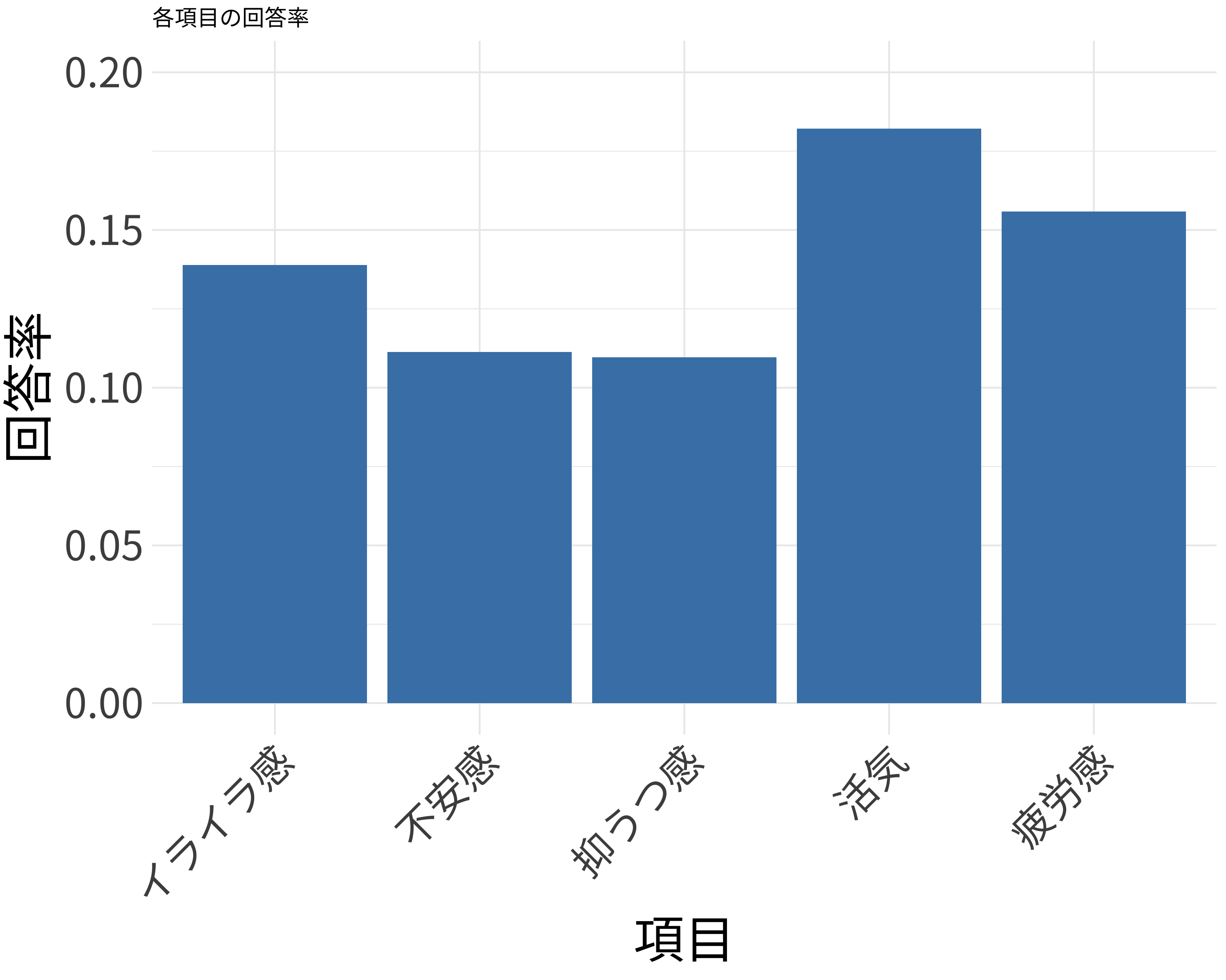
弘前データ1-4:法定検診との関係の詳細検討

3レベルに分割してしまうと見えなくなる関係性がある

著者

司馬博文

日付

5/25/2025

Modified

5/25/2025

はじめに

前項 で,BP と FLC を3レベルに離散化するよりも,連続なまま使った方が良い,そうでないと失われる情報があるのではないか?と予想した.

ここでは連続変数を用いる IRT モデルを構築してみた.すると,BP でも FLC でも識別力母数はほとんど変わらないことがわかった.

なるほど!5つの項目での,高ストレス回答確率は違い,識別力母数はそのスケールの違いを表しているだけである!

つまり項目反応モデルは完全なる null model となっており,意味のある値を学習していないようである!

library(readxl)
library(knitr)
df <- readRDS("df.rds")
dim(df)
[1] 1128   38
kable(head(df))
受付番号 受診日年齢 性別 Weight BP FLCΣ BP備考 判別式 LOX-1_H LAB_H LOX-index_H タイプ 多様性 item1 item2 item3 item4 item5 item6 item7 item8 item9 item10 item11 item12 item13 item14 item15 item16 item17 item18 BP_A_flag 年代 活気 イライラ感 疲労感 不安感 抑うつ感
2 48 2 52.7 0.47 0.81 B -3.343 75 2.2 165 B 2 2 2 2 2 2 2 4 3 2 3 2 2 2 2 1 2 3 2 0 40代 3 3 4 3 3
3 53 2 64.8 0.67 -0.30 BDG -2.727 55 2.8 154 A 1 3 1 1 1 1 2 3 3 3 2 2 2 2 2 1 1 1 1 0 50代 4 2 4 3 2
4 46 1 76.3 1.10 1.95 NA -2.974 136 3.8 517 B 2 2 3 3 2 2 2 1 1 2 2 2 1 2 2 1 1 1 1 0 40代 2 3 2 3 2
5 65 1 72.4 0.88 -8.96 D -7.338 58 2.3 133 C 2 3 3 3 2 2 2 1 1 1 2 1 1 1 1 1 1 1 1 0 60代 2 3 1 2 1
6 30 1 59.5 0.76 0.64 NA -2.776 46 2.2 101 B 2 2 2 2 3 4 3 3 3 3 4 4 3 3 3 3 3 1 1 0 30代 3 5 4 5 4
7 51 1 76.6 1.69 2.58 NA -2.377 78 3.2 250 B 2 2 2 2 2 2 2 2 2 2 2 2 2 2 1 1 1 1 1 0 50代 3 3 3 3 2
df_IRT_long <- readRDS("df_IRT_long.rds")
dim(df_IRT_long)
[1] 5640    6
kable(head(df_IRT_long))
id BP FLCΣ item response res
2 0.47 0.81 活気 3 0
2 0.47 0.81 イライラ感 3 0
2 0.47 0.81 疲労感 4 1
2 0.47 0.81 不安感 3 0
2 0.47 0.81 抑うつ感 3 0
3 0.67 -0.30 活気 4 1

1 連続説明変数の項目応答

1.1 BP の場合

library(brms)

formula_2PL_BP <- bf(
  res ~ exp(loggamma) * eta,
  loggamma ~ 1 + (1|item),
  eta ~ 1 + (1|item) + BP,
  nl = TRUE
)

BP_2PL <- brm(
  formula = formula_2PL_BP,
  data = df_IRT_long,
  family = brmsfamily("bernoulli", link = "logit"),
  chains = 4, cores = 4, iter = 8000
)

このモデルはあまりに時間を取るが,よく考えればもっと簡単に実現可能である.

比較のために,データは後の df_IRT_long_FLC に揃える.

library(brms)

formula_2PL_BP <- bf(
  res ~ (1+BP|item)
)

BP_2PL <- brm(
  formula = formula_2PL_BP,
  data = df_IRT_long_FLC,
  family = brmsfamily("bernoulli", link = "logit"),
  chains = 4, cores = 4, iter = 8000
)

saveRDS(BP_2PL, "./1-4/BP_2PL.rds")

1.1.1 識別力母数

library(ggplot2)
library(gridExtra)
library(showtext)  # 日本語フォント用のパッケージ

# 日本語フォントの設定
font_add_google("Noto Sans JP", "notosans")  # Google Fontsからフォントを追加
showtext_auto()  # 自動的にshowtextを使用するように設定
ranef_item2 <- ranef(BP_2PL)$item
posterior_means <- ranef_item2[,1,"Intercept"]
lower_bounds <- ranef_item2[,3,"Intercept"]
upper_bounds <- ranef_item2[,4,"Intercept"]
plot_df_item2 <- data.frame(
  item = rownames(ranef_item2),
  mean = posterior_means,
  lower = lower_bounds,
  upper = upper_bounds
)
p_PL2 <- ggplot(plot_df_item2, aes(x = mean, y = item)) +
  geom_point() +
  geom_errorbar(aes(xmin = lower, xmax = upper), width = 0.2) +
  theme(axis.text.x = element_text(angle = 90, hjust = 1)) +
  labs(title = NULL,
       x = "Posterior Estimate",
       y = NULL)
  #  theme(
  #   axis.text = element_text(size = 24),  # 軸の目盛りの文字サイズ
  #   axis.title = element_text(size = 30),   # 軸ラベルの文字サイズ
  #   legend.text = element_text(size = 36),  # 凡例のテキストサイズ
  #   legend.title = element_text(size = 24),  # 凡例のタイトルサイズ
  #   plot.margin = margin(r = 20)  # 右側の余白を50ポイントに設定
  # )
p_PL2

1.1.2 項目母数

ranef_item2 <- ranef(BP_2PL)$item
posterior_means <- ranef_item2[,1,"BP"]
lower_bounds <- ranef_item2[,3,"BP"]
upper_bounds <- ranef_item2[,4,"BP"]
plot_df_item2 <- data.frame(
  item = rownames(ranef_item2),
  mean = posterior_means,
  lower = lower_bounds,
  upper = upper_bounds
)
p_PL2 <- ggplot(plot_df_item2, aes(x = mean, y = item)) +
  geom_point() +
  geom_errorbar(aes(xmin = lower, xmax = upper), width = 0.2) +
  theme(axis.text.x = element_text(angle = 90, hjust = 1)) +
  labs(title = NULL,
       x = "Posterior Estimate",
       y = NULL)
p_PL2

1.2 FLCΣ の場合

df_IRT_long_FLC <- df_IRT_long[df_IRT_long$id %in% df$受付番号[is.na(df$`BP備考`)], ]
dim(df_IRT_long_FLC)
[1] 2920    6
library(brms)

formula_2PL_FLC <- bf(
  res ~ (1+FLCΣ|item)
)

FLC_2PL <- brm(
  formula = formula_2PL_FLC,
  data = df_IRT_long_FLC,
  family = brmsfamily("bernoulli", link = "logit"),
  chains = 4, cores = 4, iter = 8000
)

saveRDS(FLC_2PL, "./1-4/FLC_2PL.rds")

1.2.1 識別力母数

ranef_item2 <- ranef(FLC_2PL)$item
posterior_means <- ranef_item2[,1,"Intercept"]
lower_bounds <- ranef_item2[,3,"Intercept"]
upper_bounds <- ranef_item2[,4,"Intercept"]
plot_df_item2 <- data.frame(
  item = rownames(ranef_item2),
  mean = posterior_means,
  lower = lower_bounds,
  upper = upper_bounds
)
p_PL2 <- ggplot(plot_df_item2, aes(x = mean, y = item)) +
  geom_point() +
  geom_errorbar(aes(xmin = lower, xmax = upper), width = 0.2) +
  theme(axis.text.x = element_text(angle = 90, hjust = 1)) +
  labs(title = NULL,
       x = "Posterior Estimate",
       y = NULL)
  #  theme(
  #   axis.text = element_text(size = 24),  # 軸の目盛りの文字サイズ
  #   axis.title = element_text(size = 30),   # 軸ラベルの文字サイズ
  #   legend.text = element_text(size = 36),  # 凡例のテキストサイズ
  #   legend.title = element_text(size = 24),  # 凡例のタイトルサイズ
  #   plot.margin = margin(r = 20)  # 右側の余白を50ポイントに設定
  # )
p_PL2

1.2.2 項目母数

ranef_item2 <- ranef(FLC_2PL)$item
posterior_means <- ranef_item2[,1,"FLCΣ"]
lower_bounds <- ranef_item2[,3,"FLCΣ"]
upper_bounds <- ranef_item2[,4,"FLCΣ"]
plot_df_item2 <- data.frame(
  item = rownames(ranef_item2),
  mean = posterior_means,
  lower = lower_bounds,
  upper = upper_bounds
)
p_PL2 <- ggplot(plot_df_item2, aes(x = mean, y = item)) +
  geom_point() +
  geom_errorbar(aes(xmin = lower, xmax = upper), width = 0.2) +
  theme(axis.text.x = element_text(angle = 90, hjust = 1)) +
  labs(title = NULL,
       x = "Posterior Estimate",
       y = NULL)
p_PL2

1.3 BP と FLC の違い

loo_compare(loo(BP_2PL), loo(FLC_2PL))
        elpd_diff se_diff
BP_2PL   0.0       0.0   
FLC_2PL -1.5       2.7   

BP の方が当てはまりが良いようである.

2 項目ごとの違い

kable(head(df_IRT_long_FLC))
id BP FLCΣ item response res
4 1.10 1.95 活気 2 0
4 1.10 1.95 イライラ感 3 0
4 1.10 1.95 疲労感 2 0
4 1.10 1.95 不安感 3 0
4 1.10 1.95 抑うつ感 2 0
6 0.76 0.64 活気 3 0
res_疲労感 <- df_IRT_long_FLC$res[df_IRT_long_FLC$item == "疲労感"]
res_活気 <- df_IRT_long_FLC$res[df_IRT_long_FLC$item == "活気"]
res_抑うつ感 <- df_IRT_long_FLC$res[df_IRT_long_FLC$item == "抑うつ感"]
res_不安感 <- df_IRT_long_FLC$res[df_IRT_long_FLC$item == "不安感"]
res_イライラ感 <- df_IRT_long_FLC$res[df_IRT_long_FLC$item == "イライラ感"]
# 各項目の回答率を計算
response_rates <- c(
  mean(res_疲労感),
  mean(res_活気, na.rm = TRUE),
  mean(res_抑うつ感),
  mean(res_不安感),
  mean(res_イライラ感, na.rm = TRUE)
)

# 項目名のベクトル
item_names <- c("疲労感", "活気", "抑うつ感", "不安感", "イライラ感")

# データフレームの作成
plot_data <- data.frame(
  item = item_names,
  rate = response_rates
)

# 棒グラフの作成
ggplot(plot_data, aes(x = item, y = rate)) +
  geom_bar(stat = "identity", fill = "steelblue") +
  theme_minimal() +
  labs(
    title = "各項目の回答率",
    x = "項目",
    y = "回答率"
  ) +
  theme(
    axis.text.x = element_text(angle = 45, hjust = 1),
    text = element_text(family = "notosans"),
    axis.text = element_text(size = 24),
    axis.title = element_text(size = 30),
    legend.text = element_text(size = 36),
    legend.title = element_text(size = 24),
    # plot.margin = margin(r = 20, l = 10)
  ) +
  ylim(0, 0.2)  # y軸の範囲を0から1に設定