ココシルデータ解析１-１

昇格の影響の特定

著者

司馬博文

日付

4/26/2025

はじめに

従業員 28 名を対象に，７月と10月の２回，繰り返しココシルスコアが測定された．同時に本企業では４月と10月に異動と昇進があり，その有無も紐づけられている．しかし，初回の測定は昇進の辞令発令後３ヶ月であるのに対し，２回目の測定は辞令があった当月である．この違いを考慮したモデルを複数フィットしてみる．

基本的に説明変数は，顧客変更，部署異動，昇進の３つのみを考える．

1 検定

df_long_first <- df_long[df_long$測定時点 == 1, ]

t.test(df_long_first$スコア値[df_long_first$昇降格 == 1],
       df_long_first$スコア値[df_long_first$昇降格 == 0])


    Welch Two Sample t-test

data:  df_long_first$スコア値[df_long_first$昇降格 == 1] and df_long_first$スコア値[df_long_first$昇降格 == 0]
t = 1.6724, df = 24.042, p-value = 0.1074
alternative hypothesis: true difference in means is not equal to 0
95 percent confidence interval:
 -2.715026 25.923359
sample estimates:
mean of x mean of y 
 53.66667  42.06250

t.test(スコア値 ~ 昇降格, data = df_long_first, var.equal = TRUE)


    Two Sample t-test

data:  スコア値 by 昇降格
t = -1.6687, df = 26, p-value = 0.1072
alternative hypothesis: true difference in means between group 0 and group 1 is not equal to 0
95 percent confidence interval:
 -25.898354   2.690021
sample estimates:
mean in group 0 mean in group 1 
       42.06250        53.66667

有意差ないなあ……．

# まず昇降格が1の人のIDを取得
target_ids <- df_long_first$id[df_long_first$昇降格 == 1]

# そのIDを持つ人のデータをdf_longから抽出
df_long_promoted <- df_long[df_long$id %in% target_ids, ]

library(ggplot2)

# 基本的な時系列プロット（各個人の変化を線で結ぶ）
ggplot(df_long_promoted, aes(x = 測定時点, y = スコア値, group = id)) +
  geom_line(alpha = 1.0) +  # 個人の変化を示す線
  geom_point() +            # 各測定点
  theme_minimal() +         # シンプルなテーマ
  labs(title = "10 月昇格者のスコア値",
       x = "測定時点",
       y = "スコア値") +
  theme(
    text = element_text(family = "BIZUDGothic-Regular", size = 12),
    axis.text = element_text(size = 34),
    axis.title = element_text(size = 45),
    title = element_text(size = 45)
  ) +
  scale_x_continuous(breaks = c(0, 1), 
                    labels = c("７月", "10月（昇格当月）"))

Warning: Removed 1 row containing missing values (`geom_line()`).

Warning: Removed 1 rows containing missing values (`geom_point()`).

# 平均値の変化も追加したバージョン
# ggplot(df_long_promoted, aes(x = 測定時点, y = スコア値)) +
#   geom_line(aes(group = id), alpha = 0.3) +  # 個人の変化（薄く表示）
#   geom_point(alpha = 0.3) +                   # 個人の測定点
#   stat_summary(fun = mean, geom = "point", color = "red", size = 3) +  # 平均値
#   stat_summary(fun = mean, geom = "line", color = "red", group = 1) +  # 平均値を結ぶ線
#   theme_minimal() +
#   labs(title = "昇降格群のスコア値の変化（赤線は平均値）",
#        x = "測定時点",
#        y = "スコア値") +
#   scale_x_continuous(breaks = c(0, 1), 
#                     labels = c("1回目", "2回目"))

ggplot(df_long_promoted, aes(x = factor(測定時点), y = スコア値)) +
  geom_boxplot(width = 0.3, fill = "lightgray") +  # 箱ひげ図
  geom_line(aes(group = id), alpha = 0.3) +        # 個人の変化
  geom_point(size = 3, alpha = 0.3) +                        # 個人の測定点
  theme_minimal() +
  labs(title = "10 月昇格者のココシルスコア",
       x = "測定時点",
       y = "ココシルスコア") +
   theme(
    text = element_text(family = "BIZUDGothic-Regular", size = 11),
    axis.text = element_text(size = 30),
    axis.title = element_text(size = 40),
    title = element_text(size = 40)
  ) +
  scale_x_discrete(labels = c("昇格３ヶ月前", "昇格当月"))

Warning: Removed 1 rows containing non-finite values (`stat_boxplot()`).

Warning: Removed 1 row containing missing values (`geom_line()`).

Warning: Removed 1 rows containing missing values (`geom_point()`).

ggsave("昇格者のスコア.svg")

Saving 6 x 4 in image

Warning: Removed 1 rows containing non-finite values (`stat_boxplot()`).

Warning: Removed 1 row containing missing values (`geom_line()`).

Warning: Removed 1 rows containing missing values (`geom_point()`).

t.test(df_long_promoted$スコア値[df_long_promoted$測定時点 == 0],
       df_long_promoted$スコア値[df_long_promoted$測定時点 == 1])


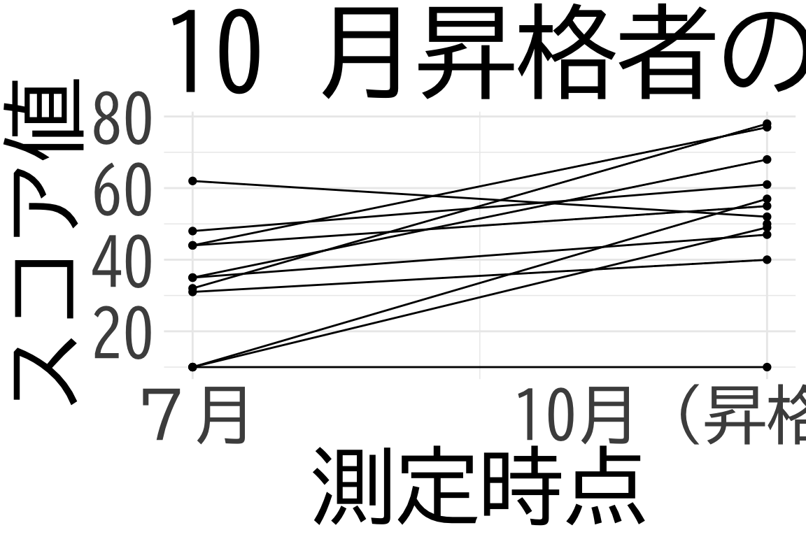
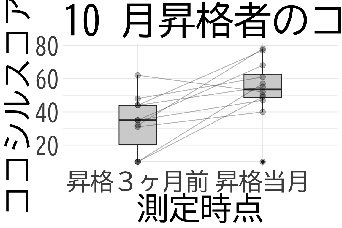
    Welch Two Sample t-test

data:  df_long_promoted$スコア値[df_long_promoted$測定時点 == 0] and df_long_promoted$スコア値[df_long_promoted$測定時点 == 1]
t = -2.848, df = 20.976, p-value = 0.00964
alternative hypothesis: true difference in means is not equal to 0
95 percent confidence interval:
 -36.073366  -5.623604
sample estimates:
mean of x mean of y 
 32.81818  53.66667

wilcox.test(スコア値 ~ 測定時点, data = df_long_promoted)

Warning in wilcox.test.default(x = DATA[[1L]], y = DATA[[2L]], ...):
タイがあるため、正確な p 値を計算することができません


    Wilcoxon rank sum test with continuity correction

data:  スコア値 by 測定時点
W = 21.5, p-value = 0.006606
alternative hypothesis: true location shift is not equal to 0

# まず昇降格が1の人のIDを取得
target_ids <- df_long_first$id[df_long_first$昇降格 == 1]

# そのIDを持つ人のデータをdf_longから抽出
df_long_not_promoted <- df_long[!(df_long$id %in% target_ids), ]

t.test(df_long_not_promoted$スコア値[df_long_not_promoted$測定時点 == 0],
       df_long_not_promoted$スコア値[df_long_not_promoted$測定時点 == 1])


    Welch Two Sample t-test

data:  df_long_not_promoted$スコア値[df_long_not_promoted$測定時点 == 0] and df_long_not_promoted$スコア値[df_long_not_promoted$測定時点 == 1]
t = -2.1173, df = 28.982, p-value = 0.04293
alternative hypothesis: true difference in means is not equal to 0
95 percent confidence interval:
 -26.2046758  -0.4536575
sample estimates:
mean of x mean of y 
 28.73333  42.06250

wilcox.test(スコア値 ~ 測定時点, data = df_long_not_promoted)

Warning in wilcox.test.default(x = DATA[[1L]], y = DATA[[2L]], ...):
タイがあるため、正確な p 値を計算することができません


    Wilcoxon rank sum test with continuity correction

data:  スコア値 by 測定時点
W = 65, p-value = 0.03018
alternative hypothesis: true location shift is not equal to 0

sum(na.omit(df_long_not_promoted[df_long_not_promoted$測定時点==1, "スコア値"] - df_long_not_promoted[df_long_not_promoted$測定時点==0, "スコア値"]))/dim(na.omit(df_long_not_promoted))[1]/2

[1] 3.290323

sum(na.omit(df_long_promoted[df_long_promoted$測定時点==1, "スコア値"] - df_long_promoted[df_long_promoted$測定時点==0, "スコア値"])/dim(na.omit(df_long_promoted)))[1]/2

[1] 7.596014

# データフレームから値を抽出する際に$演算子を使用
diff1 <- na.omit(
    df_long_not_promoted$スコア値[df_long_not_promoted$測定時点==1] - 
    df_long_not_promoted$スコア値[df_long_not_promoted$測定時点==0]
)
diff2 <- na.omit(
    df_long_promoted$スコア値[df_long_promoted$測定時点==1] - 
    df_long_promoted$スコア値[df_long_promoted$測定時点==0]
)

# 検定を実行
wilcox.test(diff1, diff2)

Warning in wilcox.test.default(diff1, diff2): タイがあるため、正確な p
値を計算することができません


    Wilcoxon rank sum test with continuity correction

data:  diff1 and diff2
W = 58, p-value = 0.2121
alternative hypothesis: true location shift is not equal to 0

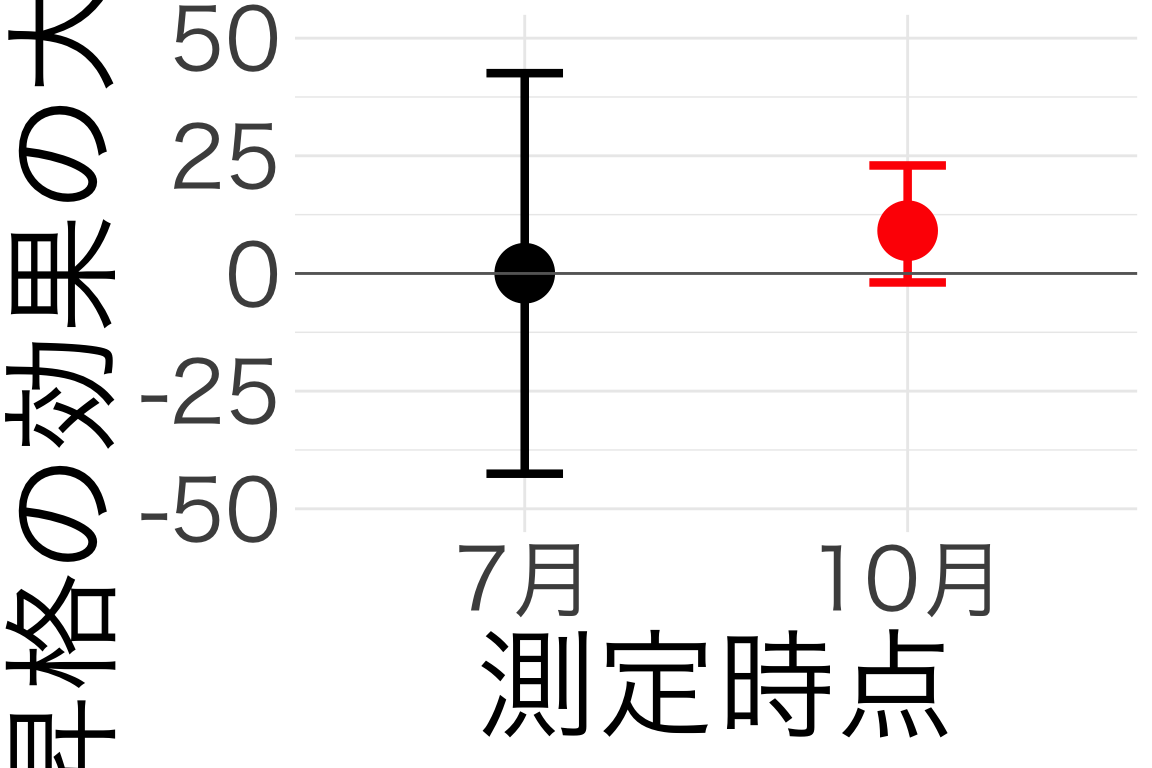
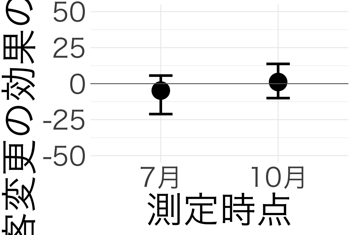
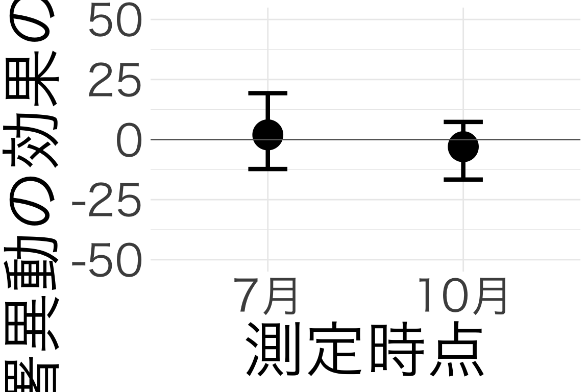
2 測定時点ごとの変動係数モデル

２回の測定で，昇降格の影響が大きく違う可能性があることがわかった．

ランダム係数の間の標準偏差がすごく大きい：\(\sigma=17.04\)．

2.1 昇降格の影響だけ変動係数にした場合

library(brms)
formula <- bf(スコア値 ~ 1 + 顧客変更 + 部署異動 + (昇降格 | 測定時点))
fit <- brm(formula, data = df_long, chains = 4, cores = 4, iter = 10000)

summary(fit)

Warning: There were 86 divergent transitions after warmup. Increasing
adapt_delta above 0.8 may help. See
http://mc-stan.org/misc/warnings.html#divergent-transitions-after-warmup

 Family: gaussian 
  Links: mu = identity; sigma = identity 
Formula: スコア値 ~ 1 + 顧客変更 + 部署異動 + (昇降格 | 測定時点) 
   Data: df_long (Number of observations: 54) 
  Draws: 4 chains, each with iter = 10000; warmup = 5000; thin = 1;
         total post-warmup draws = 20000

Multilevel Hyperparameters:
~測定時点 (Number of levels: 2) 
                      Estimate Est.Error l-95% CI u-95% CI Rhat Bulk_ESS
sd(Intercept)            13.40     10.04     1.40    39.27 1.00     7242
sd(昇降格)               15.55     12.76     0.82    49.33 1.00     8309
cor(Intercept,昇降格)     0.11      0.56    -0.91     0.96 1.00    13160
                      Tail_ESS
sd(Intercept)             5617
sd(昇降格)                6813
cor(Intercept,昇降格)    11316

Regression Coefficients:
          Estimate Est.Error l-95% CI u-95% CI Rhat Bulk_ESS Tail_ESS
Intercept    38.00      8.69    20.61    56.10 1.00     6546     5285
顧客変更     -2.44      6.37   -14.93    10.08 1.00    14820     7116
部署異動     -0.54      7.36   -14.78    14.03 1.00    15710    12255

Further Distributional Parameters:
      Estimate Est.Error l-95% CI u-95% CI Rhat Bulk_ESS Tail_ESS
sigma    18.13      1.85    14.98    22.20 1.00    16138    12716

Draws were sampled using sampling(NUTS). For each parameter, Bulk_ESS
and Tail_ESS are effective sample size measures, and Rhat is the potential
scale reduction factor on split chains (at convergence, Rhat = 1).

print(ranef(fit))

$測定時点
, , Intercept

   Estimate Est.Error      Q2.5    Q97.5
0 -5.909091  8.719841 -24.82095 11.21010
1  5.094694  8.583053 -11.48179 23.90954

, , 昇降格

     Estimate Est.Error       Q2.5    Q97.5
0 0.009877498 19.434528 -41.289913 40.83618
1 8.357619973  6.856646  -2.602692 22.76199

2.2 昇降格の変動係数のプロット

library(brms)
formula <- bf(スコア値 ~ (1 + 昇降格 | 測定時点))
fit <- brm(formula, data = df_long, chains = 4, cores = 4, iter = 10000)

library(ggplot2)
ranef_昇降格 <- ranef(fit)$測定時点
posterior_means <- ranef_昇降格[,1,2]
lower_bounds <- ranef_昇降格[,3,2]
upper_bounds <- ranef_昇降格[,4,2]
plot_df_昇降格 <- data.frame(
  term = rownames(ranef_昇降格),
  mean = posterior_means,
  lower = lower_bounds,
  upper = upper_bounds
)
# termを因子型に変換（順序を保持するため）
plot_df_昇降格$term <- factor(plot_df_昇降格$term, 
                           levels = c("0", "1"), 
                           labels = c("7月", "10月"))

ggplot(plot_df_昇降格, aes(x = factor(term), y = mean)) +
  geom_point(aes(color = term == "10月"), size = 10) +
  geom_errorbar(aes(ymin = lower, ymax = upper, 
                    color = term == "10月"),  # 条件による色分け
                width = 0.2, linewidth = 1.5) +
  geom_hline(yintercept = 0, color = "gray40", linewidth = 0.5) +
  theme_minimal() +
  labs(x = "測定時点", y = "昇格の効果の大きさ") +
  scale_color_manual(values = c("black", "red"), guide = "none") +  # ガイド（凡例）を非表示
  theme(
    axis.title.x = element_text(size = 45),      # x軸ラベルのサイズ
    axis.title.y = element_text(size = 45),      # y軸ラベルのサイズ
    axis.text.x = element_text(size = 32),       # x軸目盛りのサイズ
    axis.text.y = element_text(size = 32),       # y軸目盛りのサイズ
  text = element_text(family = "HiraginoSans-W3")
  ) +
  coord_cartesian(ylim = c(-50, 50))  # y軸の範囲を調整

# ggsave("昇格.png", bg="white")

2.3 すごい！じゃあ顧客変更は？

library(brms)
formula <- bf(スコア値 ~ (1 + 顧客変更 | 測定時点))
fit <- brm(formula, data = df_long, chains = 4, cores = 4, iter = 10000)

library(ggplot2)
ranef_顧客変更 <- ranef(fit)$測定時点
posterior_means <- ranef_顧客変更[,1,2]
lower_bounds <- ranef_顧客変更[,3,2]
upper_bounds <- ranef_顧客変更[,4,2]
plot_df_顧客変更 <- data.frame(
  term = rownames(ranef_顧客変更),
  mean = posterior_means,
  lower = lower_bounds,
  upper = upper_bounds
)
# termを因子型に変換（順序を保持するため）
plot_df_顧客変更$term <- factor(plot_df_顧客変更$term, 
                           levels = c("0", "1"), 
                           labels = c("7月", "10月"))

ggplot(plot_df_顧客変更, aes(x = factor(term), y = mean)) +
  geom_point(size = 10) +  # 平均値のポイント
  geom_errorbar(aes(ymin = lower, ymax = upper), width = 0.2, linewidth = 1.5) +  # エラーバー
  geom_hline(yintercept = 0, color = "gray40", linewidth = 0.5) +
  theme_minimal() +
  labs(x = "測定時点", y = "顧客変更の効果の大きさ") +
  theme(
    axis.title.x = element_text(size = 45),      # x軸ラベルのサイズ
    axis.title.y = element_text(size = 45),      # y軸ラベルのサイズ
    axis.text.x = element_text(size = 32),       # x軸目盛りのサイズ
    axis.text.y = element_text(size = 32),       # y軸目盛りのサイズ
  text = element_text(family = "HiraginoSans-W3")
  ) +
  coord_cartesian(ylim = c(-50, 50))  # y軸の範囲を調整

# ggsave("顧客変更.png", bg="white")

2.4 すごい！続けて部署異動は？

library(brms)
formula <- bf(スコア値 ~ (1 + 部署異動 | 測定時点))
fit <- brm(formula, data = df_long, chains = 4, cores = 4, iter = 10000)

library(ggplot2)
ranef_部署異動 <- ranef(fit)$測定時点
posterior_means <- ranef_部署異動[,1,2]
lower_bounds <- ranef_部署異動[,3,2]
upper_bounds <- ranef_部署異動[,4,2]
plot_df_部署異動 <- data.frame(
  term = rownames(ranef_部署異動),
  mean = posterior_means,
  lower = lower_bounds,
  upper = upper_bounds
)
# termを因子型に変換（順序を保持するため）
plot_df_部署異動$term <- factor(plot_df_部署異動$term, 
                           levels = c("0", "1"), 
                           labels = c("7月", "10月"))

ggplot(plot_df_部署異動, aes(x = factor(term), y = mean)) +
  geom_point(size = 10) +  # 平均値のポイント
  geom_errorbar(aes(ymin = lower, ymax = upper), width = 0.2, linewidth = 1.5) +  # エラーバー
  geom_hline(yintercept = 0, color = "gray40", linewidth = 0.5) +
  theme_minimal() +
  labs(x = "測定時点", y = "部署異動の効果の大きさ") +
  theme(
    axis.title.x = element_text(size = 45),      # x軸ラベルのサイズ
    axis.title.y = element_text(size = 45),      # y軸ラベルのサイズ
    axis.text.x = element_text(size = 32),       # x軸目盛りのサイズ
    axis.text.y = element_text(size = 32),       # y軸目盛りのサイズ
  text = element_text(family = "HiraginoSans-W3")
  ) +
  coord_cartesian(ylim = c(-50, 50))  # y軸の範囲を調整

# ggsave("部署異動.png", bg="white")

2.5 ちょっと prior を検証したくなった

get_prior(formula, data = df_long)

Warning: Rows containing NAs were excluded from the model.

                  prior     class      coef    group resp dpar nlpar lb ub
                 lkj(1)       cor                                         
                 lkj(1)       cor           測定時点                      
 student_t(3, 39, 17.8) Intercept                                         
  student_t(3, 0, 17.8)        sd                                     0   
  student_t(3, 0, 17.8)        sd           測定時点                  0   
  student_t(3, 0, 17.8)        sd Intercept 測定時点                  0   
  student_t(3, 0, 17.8)        sd  部署異動 測定時点                  0   
  student_t(3, 0, 17.8)     sigma                                     0   
       source
      default
 (vectorized)
      default
      default
 (vectorized)
 (vectorized)
 (vectorized)
      default

2.6 頻度論的な検定もしてみたい

t.test(スコア値 ~ 測定時点, data = df_long)


    Welch Two Sample t-test

data:  スコア値 by 測定時点
t = -3.4348, df = 51.89, p-value = 0.001174
alternative hypothesis: true difference in means between group 0 and group 1 is not equal to 0
95 percent confidence interval:
 -26.257600  -6.890752
sample estimates:
mean in group 0 mean in group 1 
       30.46154        47.03571

2.7 全て変動係数にした場合

library(brms)
formula <- bf(スコア値 ~ (1 + 顧客変更 + 部署異動 + 昇降格 | 測定時点))
fit <- brm(formula, data = df_long, chains = 4, cores = 4, iter = 10000)

summary(fit)

Warning: There were 111 divergent transitions after warmup. Increasing
adapt_delta above 0.8 may help. See
http://mc-stan.org/misc/warnings.html#divergent-transitions-after-warmup

 Family: gaussian 
  Links: mu = identity; sigma = identity 
Formula: スコア値 ~ (1 + 顧客変更 + 部署異動 + 昇降格 | 測定時点) 
   Data: df_long (Number of observations: 54) 
  Draws: 4 chains, each with iter = 10000; warmup = 5000; thin = 1;
         total post-warmup draws = 20000

Multilevel Hyperparameters:
~測定時点 (Number of levels: 2) 
                        Estimate Est.Error l-95% CI u-95% CI Rhat Bulk_ESS
sd(Intercept)              12.58      9.74     0.86    37.60 1.00     7362
sd(顧客変更)               10.60      9.35     0.42    34.48 1.00    10133
sd(部署異動)                9.37      9.83     0.33    32.83 1.00    10214
sd(昇降格)                 16.80     13.66     1.05    52.09 1.00     9434
cor(Intercept,顧客変更)     0.08      0.44    -0.76     0.85 1.00    15044
cor(Intercept,部署異動)    -0.05      0.44    -0.83     0.78 1.00    19759
cor(顧客変更,部署異動)     -0.03      0.45    -0.83     0.80 1.00    15836
cor(Intercept,昇降格)       0.07      0.44    -0.76     0.83 1.00    15226
cor(顧客変更,昇降格)        0.06      0.44    -0.78     0.84 1.00    14599
cor(部署異動,昇降格)       -0.02      0.45    -0.82     0.80 1.00    13589
                        Tail_ESS
sd(Intercept)               6830
sd(顧客変更)                8109
sd(部署異動)                7919
sd(昇降格)                  7091
cor(Intercept,顧客変更)    12853
cor(Intercept,部署異動)    12946
cor(顧客変更,部署異動)     14607
cor(Intercept,昇降格)      12694
cor(顧客変更,昇降格)       13632
cor(部署異動,昇降格)       15194

Regression Coefficients:
          Estimate Est.Error l-95% CI u-95% CI Rhat Bulk_ESS Tail_ESS
Intercept    37.68      7.91    21.85    54.69 1.00     6710     8195

Further Distributional Parameters:
      Estimate Est.Error l-95% CI u-95% CI Rhat Bulk_ESS Tail_ESS
sigma    17.78      1.79    14.69    21.62 1.00    17831    13424

Draws were sampled using sampling(NUTS). For each parameter, Bulk_ESS
and Tail_ESS are effective sample size measures, and Rhat is the potential
scale reduction factor on split chains (at convergence, Rhat = 1).

print(ranef(fit))

$測定時点
, , Intercept

   Estimate Est.Error      Q2.5    Q97.5
0 -5.214108  8.150085 -23.46991 10.18071
1  4.243538  8.050756 -11.47130 22.49473

, , 顧客変更

   Estimate Est.Error       Q2.5    Q97.5
0 -5.203859  6.846780 -21.181843  5.70881
1  2.988036  6.037004  -7.517553 17.17517

, , 部署異動

   Estimate Est.Error      Q2.5     Q97.5
0  1.505993  7.049372 -12.20847 18.163898
1 -1.910259  5.598964 -14.84205  8.655186

, , 昇降格

    Estimate Est.Error       Q2.5    Q97.5
0 0.05449668 20.186178 -40.472147 43.88947
1 9.17204662  6.842582  -2.096607 23.21416

3 固定効果モデル（従来の分析）

library(brms)
formula <- bf(スコア値 ~ (1|id) + 測定時点 + 顧客変更 + 部署異動 + 昇降格)
fit <- brm(formula, data = df_long, chains = 4, cores = 4)

summary(fit)

Warning: There were 4 divergent transitions after warmup. Increasing
adapt_delta above 0.8 may help. See
http://mc-stan.org/misc/warnings.html#divergent-transitions-after-warmup

 Family: gaussian 
  Links: mu = identity; sigma = identity 
Formula: スコア値 ~ (1 | id) + 測定時点 + 顧客変更 + 部署異動 + 昇降格 
   Data: df_long (Number of observations: 54) 
  Draws: 4 chains, each with iter = 2000; warmup = 1000; thin = 1;
         total post-warmup draws = 4000

Multilevel Hyperparameters:
~id (Number of levels: 28) 
              Estimate Est.Error l-95% CI u-95% CI Rhat Bulk_ESS Tail_ESS
sd(Intercept)     9.06      3.92     1.18    16.74 1.00      809     1343

Regression Coefficients:
          Estimate Est.Error l-95% CI u-95% CI Rhat Bulk_ESS Tail_ESS
Intercept    30.53      3.86    23.02    38.21 1.00     3228     2771
測定時点     12.01      5.44     1.06    22.70 1.00     3282     2449
顧客変更     -0.48      6.47   -13.27    12.18 1.00     3318     2804
部署異動      0.38      6.90   -13.03    13.87 1.00     4063     3082
昇降格       10.61      7.16    -3.27    24.51 1.00     2841     2502

Further Distributional Parameters:
      Estimate Est.Error l-95% CI u-95% CI Rhat Bulk_ESS Tail_ESS
sigma    15.47      2.23    11.63    20.34 1.00      994     1805

Draws were sampled using sampling(NUTS). For each parameter, Bulk_ESS
and Tail_ESS are effective sample size measures, and Rhat is the potential
scale reduction factor on split chains (at convergence, Rhat = 1).