弘前データ６：法定検診項目＋ストレスチェックにより，A タイプを見分ける方法

著者

司馬博文

日付

8/13/2025

備考は全て外し，LOX_Index と 判別式 も説明変数としては考慮しない．

age	sex	Weight	LOX	LAB	type	BMI	med	RedBloodCell	Hemoglobin	HbA1c	AST	ALT	gammaGT	TotalCholesterol	TG	BloodSugar	HDL	LDL	UrineSugar	SystolicBP	DiastolicBP	drink	smoke	exercise	breakfast	活気	イライラ感	疲労感	不安感	抑うつ感
64	2	54.2	86	2.6	B	22.8	2	438	13.0	5.8	24	23	70	243	70	96	93	135	-1	151	97	0	0	4	2	3	1	1	1	1
48	2	52.7	75	2.2	B	22.1	2	452	14.0	5.5	23	18	25	282	64	91	97	171	-1	131	85	2	1	4	2	3	3	4	3	3
53	2	64.8	55	2.8	A	26.0	2	464	13.9	5.5	16	14	19	262	106	99	69	171	-1	109	75	0	0	2	2	4	2	4	3	2
46	1	76.3	136	3.8	B	26.0	2	553	16.3	5.9	17	16	56	221	148	107	50	139	-1	132	95	2	2	1	2	2	3	2	3	2
65	1	72.4	58	2.3	C	26.2	2	520	16.4	5.4	16	10	28	201	97	90	77	104	-1	136	88	2	2	3	2	2	3	1	2	1
30	1	59.5	46	2.2	B	19.5	2	555	16.0	5.2	18	18	26	185	169	89	49	103	-1	120	73	0	0	1	2	3	5	4	5	4

1 CART モデル

library(rpart)

Warning: パッケージ 'rpart' はバージョン 4.3.3 の R の下で造られました

library(rpart.plot)

Warning: パッケージ 'rpart.plot' はバージョン 4.3.3 の R の下で造られました

# 目的変数が5クラスになっても、式は同じ
# rpartが自動で多クラス分類として扱ってくれる
cart_model_5class <- rpart(
  type ~ .,        # 目的変数を5クラスのものに変更
  data = df_filtered,
  method = "class",       # 分類なので "class" のまま
  control = rpart.control(cp = 0.001)
)
printcp(cart_model_5class)


Classification tree:
rpart(formula = type ~ ., data = df_filtered, method = "class", 
    control = rpart.control(cp = 0.001))

Variables actually used in tree construction:
 [1] age              ALT              BloodSugar       BMI             
 [5] DiastolicBP      drink            exercise         gammaGT         
 [9] HbA1c            HDL              Hemoglobin       LAB             
[13] LDL              LOX              RedBloodCell     sex             
[17] SystolicBP       TG               TotalCholesterol Weight          
[21] 不安感           抑うつ感        

Root node error: 359/1136 = 0.31602

n=1136 ( 26 個の観測値が欠損のため削除されました )

         CP nsplit rel error xerror     xstd
1 0.0069638      0   1.00000 1.0000 0.043649
2 0.0055710     14   0.87744 1.0891 0.044605
3 0.0046425     22   0.83008 1.1114 0.044816
4 0.0041783     25   0.81616 1.1142 0.044842
5 0.0027855     31   0.78552 1.1309 0.044993
6 0.0018570     33   0.77994 1.1866 0.045452
7 0.0010000     36   0.77437 1.2061 0.045597

# 決定木を可視化
rpart.plot(
  cart_model_5class,
  type = 4,
  extra = 104,           # 各ノードのクラス別サンプル数を表示
  box.palette = "auto",  # 色を自動で設定
  shadow.col = "gray",
  nn = TRUE
)

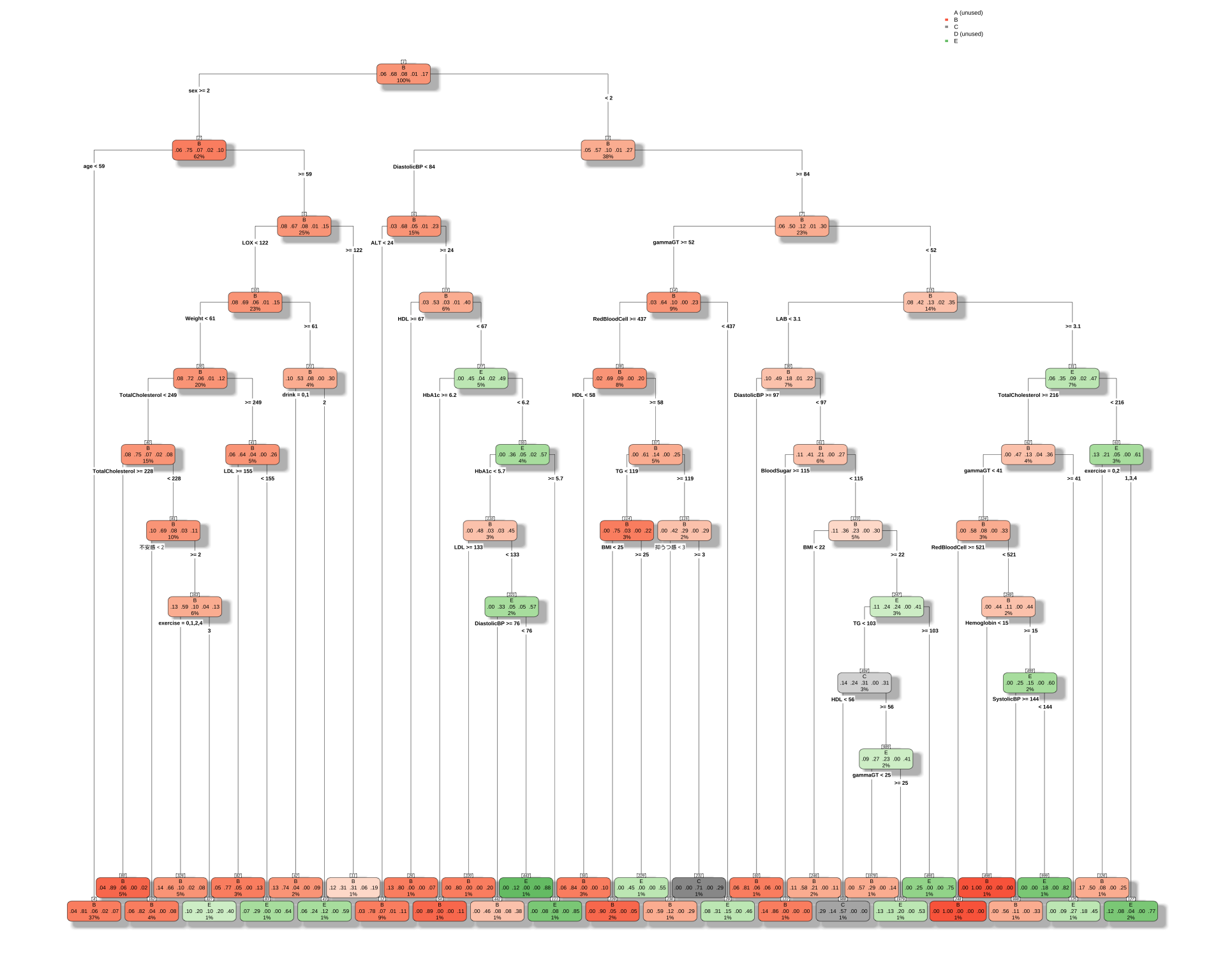
やはり最初から「女性ならばほとんど Type B だ」と決めつけている．

2 男女で違う CART モデルを推定する

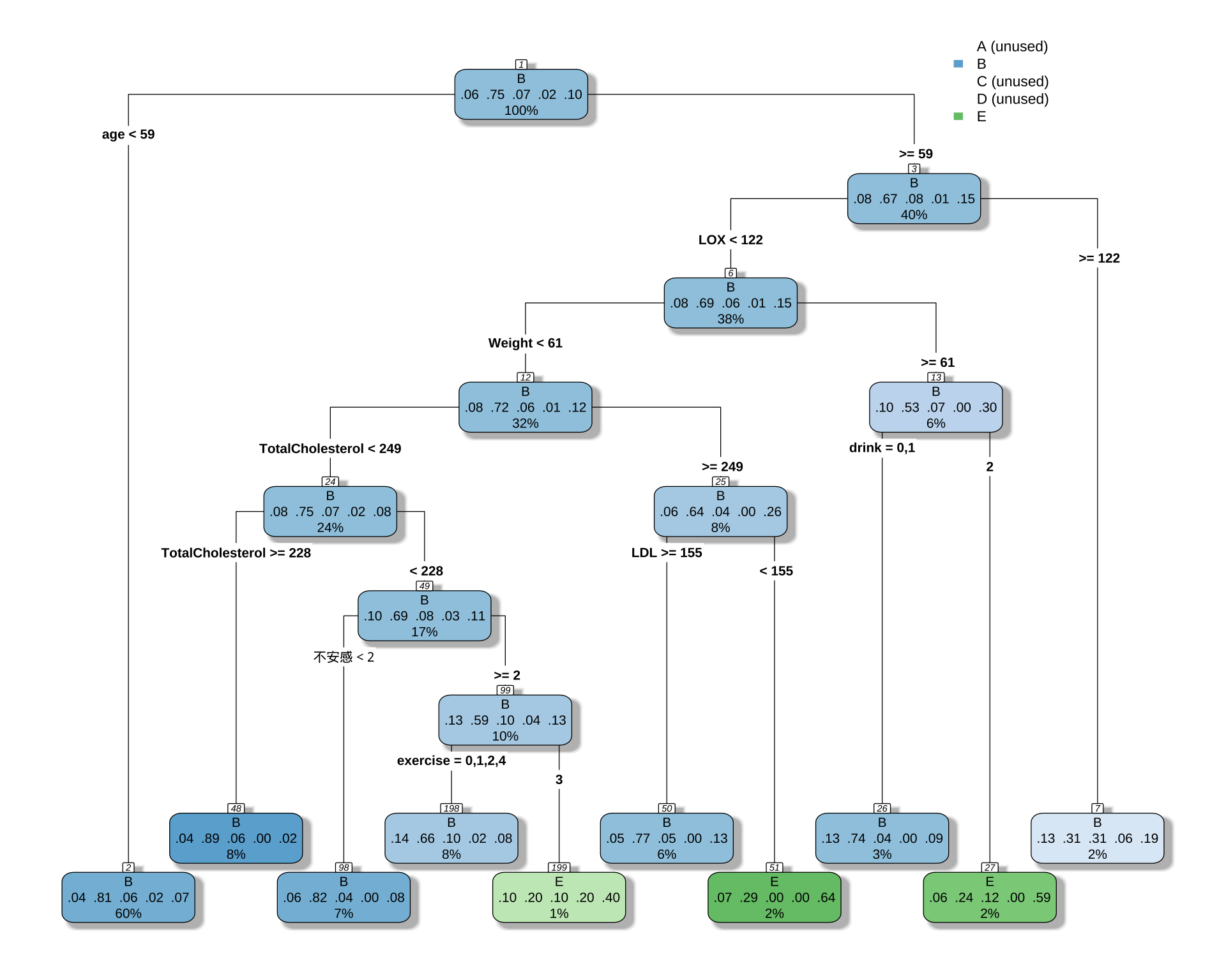
男性の場合正答率が６割しか出ないが，女性の場合は８割出る．これは女性の方に C, E type がないためである．

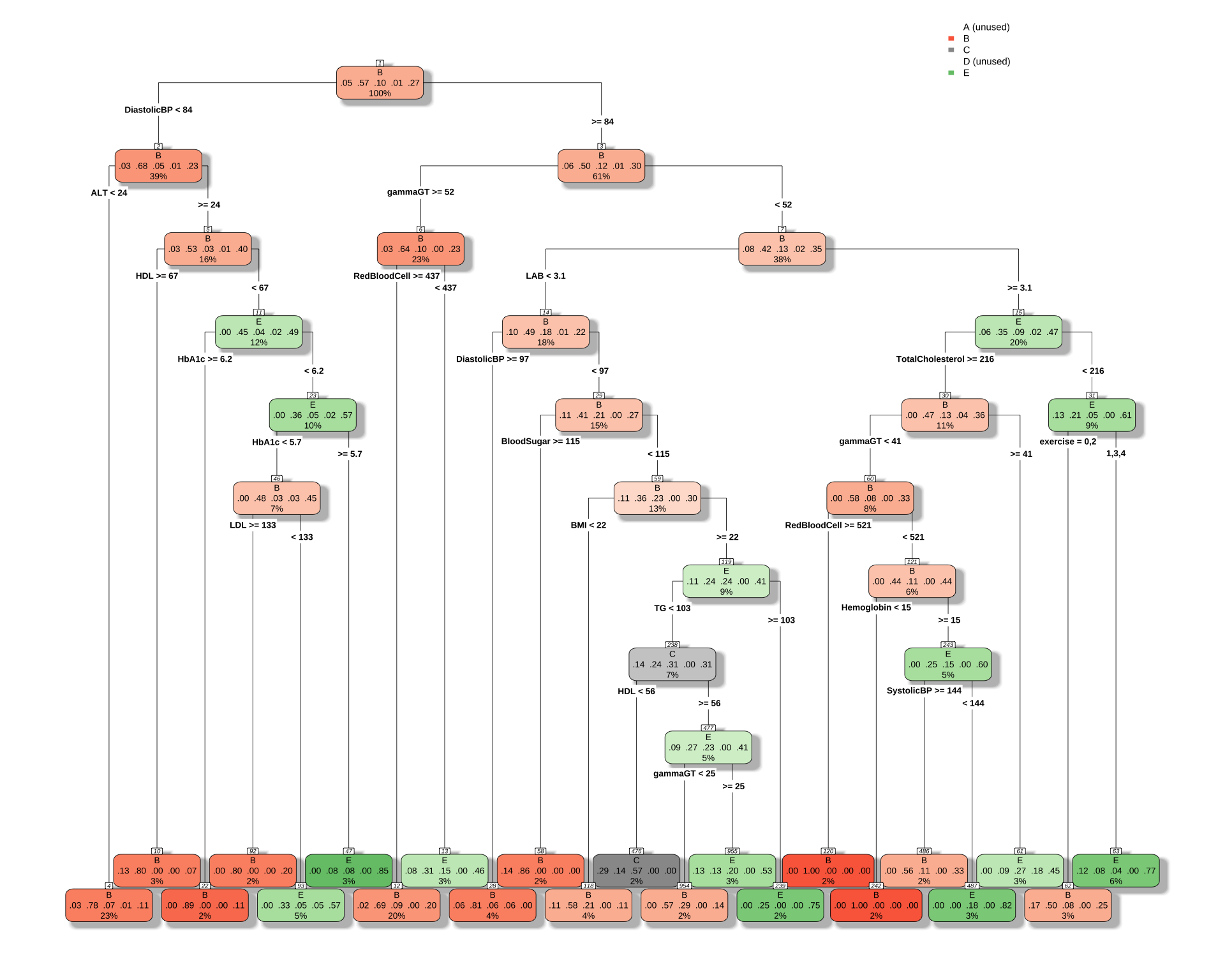
2.1 男性の場合

「 BMI が小さくて多様性が３ならば A タイプ」というルールは変わらないようである．

library(rpart)
library(rpart.plot)

df_male <- df_filtered %>%
  filter(sex == 1)

# 目的変数が5クラスになっても、式は同じ
# rpartが自動で多クラス分類として扱ってくれる
cart_model_5class <- rpart(
  type ~ .,        # 目的変数を5クラスのものに変更
  data = df_male,
  method = "class"
)
printcp(cart_model_5class)


Classification tree:
rpart(formula = type ~ ., data = df_male, method = "class")

Variables actually used in tree construction:
 [1] ALT              BloodSugar       BMI              DiastolicBP     
 [5] exercise         gammaGT          HbA1c            HDL             
 [9] Hemoglobin       LAB              LDL              RedBloodCell    
[13] SystolicBP       TG               TotalCholesterol

Root node error: 185/431 = 0.42923

n=431 ( 15 個の観測値が欠損のため削除されました )

        CP nsplit rel error xerror     xstd
1 0.018018      0   1.00000 1.0000 0.055545
2 0.016216      7   0.85946 1.1568 0.056108
3 0.010811     13   0.76216 1.2270 0.056030
4 0.010000     21   0.67027 1.2703 0.055879

# 決定木を可視化
rpart.plot(
  cart_model_5class,
  type = 4,
  extra = 104,           # 各ノードのクラス別サンプル数を表示
  box.palette = "auto",  # 色を自動で設定
  shadow.col = "gray",
  nn = TRUE
)

# 予測値を取得
predictions <- predict(cart_model_5class, newdata = df_male, type = "class")

# 混同行列を作成
confusion_matrix <- table(Actual = df_male$type, Predicted = predictions)
print(confusion_matrix)

      Predicted
Actual   A   B   C   D   E
     A   0  13   2   0   6
     B   0 226   1   0  19
     C   0  24   4   0  13
     D   0   2   0   0   3
     E   0  41   0   0  77

# 正答率を計算
accuracy <- sum(predictions == df_male$type, na.rm = TRUE) / sum(!is.na(df_male$type))
cat("正答率:", round(accuracy * 100, 2), "%\n")

正答率: 71.23 %

58% の正解率が 71% になる．

2.2 女性の場合

library(rpart)
library(rpart.plot)

df_female <- df_filtered %>%
  filter(sex == 2)

# 目的変数が5クラスになっても、式は同じ
# rpartが自動で多クラス分類として扱ってくれる
cart_model_5class <- rpart(
  type ~ .,        # 目的変数を5クラスのものに変更
  data = df_female,
  method = "class",
  control = rpart.control(cp = 0.001)
)
printcp(cart_model_5class)


Classification tree:
rpart(formula = type ~ ., data = df_female, method = "class", 
    control = rpart.control(cp = 0.001))

Variables actually used in tree construction:
[1] age              drink            exercise         LDL             
[5] LOX              TotalCholesterol Weight           不安感          

Root node error: 174/705 = 0.24681

n=705 ( 11 個の観測値が欠損のため削除されました )

         CP nsplit rel error xerror     xstd
1 0.0086207      0   1.00000 1.0000 0.065793
2 0.0038314      6   0.93678 1.1897 0.069495
3 0.0010000      9   0.92529 1.2529 0.070526

# 決定木を可視化
rpart.plot(
  cart_model_5class,
  type = 4,
  extra = 104,           # 各ノードのクラス別サンプル数を表示
  box.palette = "auto",  # 色を自動で設定
  shadow.col = "gray",
  nn = TRUE
)

# 予測値を取得
predictions <- predict(cart_model_5class, newdata = df_female, type = "class")

# 混同行列を作成
confusion_matrix <- table(Actual = df_female$type, Predicted = predictions)
print(confusion_matrix)

      Predicted
Actual   A   B   C   D   E
     A   0  39   0   0   3
     B   0 521   0   0  10
     C   0  44   0   0   3
     D   0   9   0   0   2
     E   0  51   0   0  23

# 正答率を計算
accuracy <- sum(predictions == df_female$type, na.rm = TRUE) / sum(!is.na(df_female$type))
cat("正答率:", round(accuracy * 100, 2), "%\n")

正答率: 77.16 %

少ない変数でやったときはタイプ B 259 人から，261 人になっただけだったが，今回はもう少し増えるようだ．