弘前データ５：BART によるフローラ多様性予測

著者

司馬博文

日付

8/11/2025

library(readxl)
library(knitr)
df <- readRDS("df.rds")
library(showtext)
showtext_auto()

備考は全て外し，LOX_Index と 判別式 も説明変数としては考慮しない．

library(dplyr)
df_filtered <- df %>%
  filter(is.na(BP備考)) %>%
  select(-c(BP備考, LOX_Index, 判別式, id, med_col, 年代)) %>%
  droplevels()

1 CART モデル

library(rpart)
library(rpart.plot)

# 目的変数が5クラスになっても、式は同じ
# rpartが自動で多クラス分類として扱ってくれる
cart_model <- rpart(
  diversity ~ .,        # 目的変数を5クラスのものに変更
  data = df_filtered,
  method = "class"       # 分類なので "class" のまま
)
printcp(cart_model)


Classification tree:
rpart(formula = diversity ~ ., data = df_filtered, method = "class")

Variables actually used in tree construction:
[1] age      BMI      BP       LAB      type     Weight   抑うつ感

Root node error: 192/570 = 0.33684

n=570 (14 observations deleted due to missingness)

        CP nsplit rel error xerror     xstd
1 0.016927      0   1.00000 1.0000 0.058770
2 0.010417      4   0.93229 1.1250 0.060324
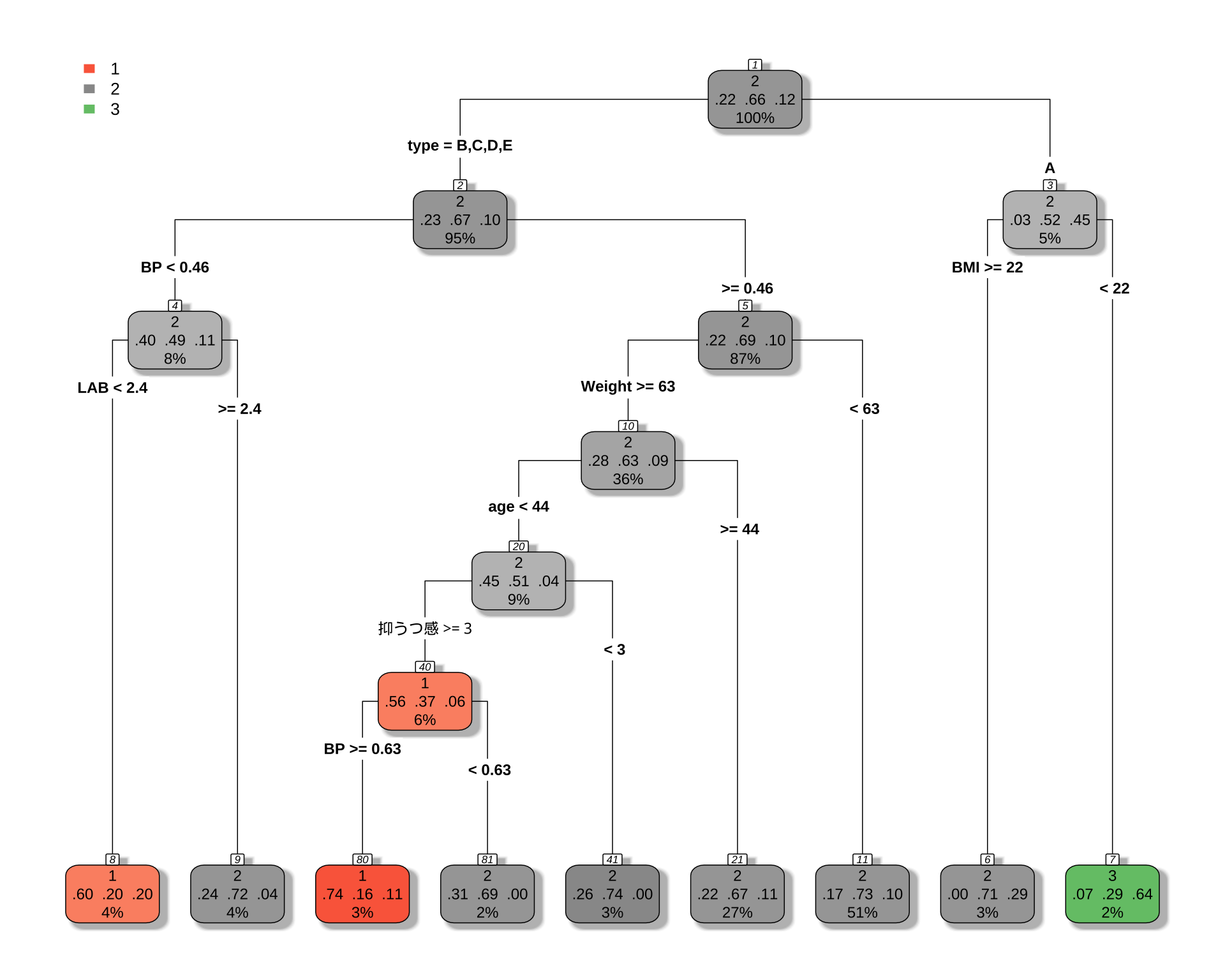
3 0.010000      8   0.87500 1.1354 0.060431

# 決定木を可視化
rpart.plot(
  cart_model,
  type = 4,
  extra = 104,           # 各ノードのクラス別サンプル数を表示
  box.palette = "auto",  # 色を自動で設定
  shadow.col = "gray",
  nn = TRUE
)

# 予測値を取得
predictions <- predict(cart_model, newdata = df_filtered, type = "class")

# 混同行列を作成
confusion_matrix <- table(Actual = df_filtered$diversity, Predicted = predictions)
print(confusion_matrix)

      Predicted
Actual   1   2   3
     1  26  99   1
     2   7 367   4
     3   6  51   9

# 正答率を計算
accuracy <- sum(predictions == df_filtered$diversity, na.rm = TRUE) / sum(!is.na(df_filtered$diversity))
cat("正答率:", round(accuracy * 100, 2), "%\n")

正答率: 70.53 %

2 男女で違う CART モデルを推定する

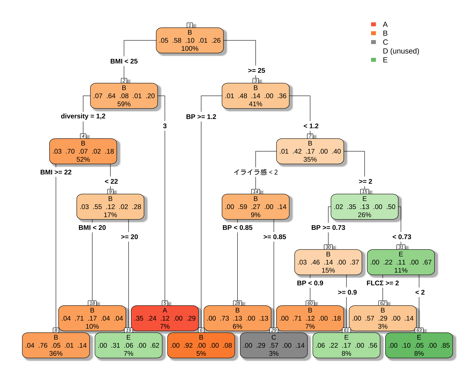
男性の場合正答率が６割しか出ないが，女性の場合は８割出る．これは女性の方に C, E type がないためである．

2.1 男性の場合

「 BMI が小さくて多様性が３ならば A タイプ」というルールは変わらないようである．

library(rpart)
library(rpart.plot)

df_male <- df_filtered %>%
  filter(sex == 1)

# 目的変数が5クラスになっても、式は同じ
# rpartが自動で多クラス分類として扱ってくれる
cart_model_5class <- rpart(
  type ~ .,        # 目的変数を5クラスのものに変更
  data = df_male,
  method = "class"       # 分類なので "class" のまま
)
printcp(cart_model_5class)


Classification tree:
rpart(formula = type ~ ., data = df_male, method = "class")

Variables actually used in tree construction:
[1] BMI        BP         diversity  FLCΣ       イライラ感

Root node error: 101/239 = 0.42259

n=239 (10 observations deleted due to missingness)

        CP nsplit rel error xerror     xstd
1 0.029703      0   1.00000 1.0000 0.075610
2 0.023102      6   0.79208 1.0594 0.076113
3 0.019802      9   0.72277 1.0198 0.075800
4 0.010000     10   0.70297 1.0297 0.075886

# 決定木を可視化
rpart.plot(
  cart_model_5class,
  type = 4,
  extra = 104,           # 各ノードのクラス別サンプル数を表示
  box.palette = "auto",  # 色を自動で設定
  shadow.col = "gray",
  nn = TRUE
)

# 予測値を取得
predictions <- predict(cart_model_5class, newdata = df_male, type = "class")

# 混同行列を作成
confusion_matrix <- table(Actual = df_male$type, Predicted = predictions)
print(confusion_matrix)

      Predicted
Actual   A   B   C   D   E
     A   6   4   0   0   1
     B   4 121   2   0  11
     C   2  14   4   0   5
     D   0   2   0   0   0
     E   5  20   1   0  37

# 正答率を計算
accuracy <- sum(predictions == df_male$type, na.rm = TRUE) / sum(!is.na(df_male$type))
cat("正答率:", round(accuracy * 100, 2), "%\n")

正答率: 70.29 %

58% の正解率が 71% になる．

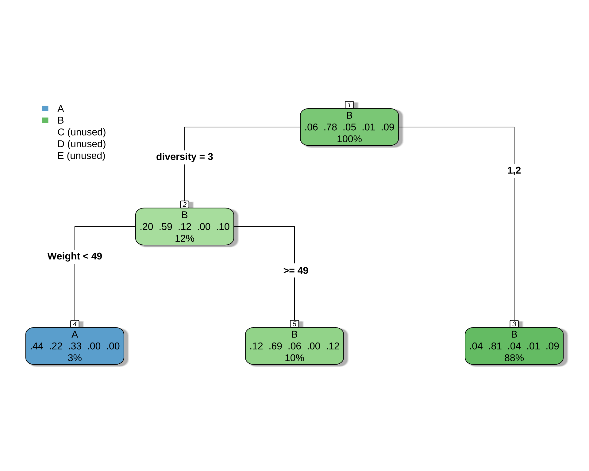
2.2 女性の場合

library(rpart)
library(rpart.plot)

df_female <- df_filtered %>%
  filter(sex == 2)

# 目的変数が5クラスになっても、式は同じ
# rpartが自動で多クラス分類として扱ってくれる
cart_model_5class <- rpart(
  type ~ .,        # 目的変数を5クラスのものに変更
  data = df_female,
  method = "class"       # 分類なので "class" のまま
)
printcp(cart_model_5class)


Classification tree:
rpart(formula = type ~ ., data = df_female, method = "class")

Variables actually used in tree construction:
[1] diversity Weight   

Root node error: 72/331 = 0.21752

n=331 (4 observations deleted due to missingness)

        CP nsplit rel error xerror    xstd
1 0.013889      0   1.00000 1.0000 0.10425
2 0.010000      2   0.97222 1.0556 0.10627

# 決定木を可視化
rpart.plot(
  cart_model_5class,
  type = 4,
  extra = 104,           # 各ノードのクラス別サンプル数を表示
  box.palette = "auto",  # 色を自動で設定
  shadow.col = "gray",
  nn = TRUE
)

# 予測値を取得
predictions <- predict(cart_model_5class, newdata = df_female, type = "class")

# 混同行列を作成
confusion_matrix <- table(Actual = df_female$type, Predicted = predictions)
print(confusion_matrix)

      Predicted
Actual   A   B   C   D   E
     A   4  16   0   0   0
     B   2 257   0   0   0
     C   3  15   0   0   0
     D   0   4   0   0   0
     E   0  30   0   0   0

# 正答率を計算
accuracy <- sum(predictions == df_female$type, na.rm = TRUE) / sum(!is.na(df_female$type))
cat("正答率:", round(accuracy * 100, 2), "%\n")

正答率: 78.85 %

これは正答の個数が，タイプ B 259 人から，261 人になっただけ．